
I/Q Measurement Panel: Receiver Settings
This tab allows to define the I/Q measurement settings and the I/Q data analysis (CCDF, ACPR, Dynamic AMAM/AMPM):
Trace display
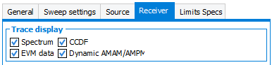
- Spectrum : display the spectrum trace of the waveform
- CCDF : display CCDF trace of the waveform
- EVM data : calculate EVM for the selected waveform (only available with PSK&QAM / LTE Downlink / NR 5G waveforms generated with the waveform generator)
- Dynamic AMAM/AMPM : display AMAM /AMPM of the waveform.
I/Q Data
- Sample rate: sets the sampling rate used during the I/Q
analysisNote: The Sampling rate value must be higher than the one defined in the I/Q Measurement Panel: Source Setting. It is recommanded to use a multiplying factor (x2,x3,x4) of the generated wavefom sampling rate to avoid heavy calculations and help the time-domain alignement algorithm to converge.
- Time: Select a time slice of the waveform.
- Measurement interval: sets the width of the waveform to
acquire. This can reduce the measurement time significantly.Note: In "Auto" mode, the "Measurement interval" will be adjusted to reach the same PAPR compared to the full waveform.
- Measurement delay; sets the delay to apply to the measurement
window. A circular shifting is performed on the waveform so that the
delay can be close to the end with a large acquisition, not
impacting on the measurement.Note: This window will be centered on the waveform max power value if it is set to "Auto".Note: This feature is also usefull to analyze a particular waveform burst when TDD waveforms are used.
- Measurement interval: sets the width of the waveform to
acquire. This can reduce the measurement time significantly.
- Sub-fremas: Select a specific number of sub-frames of the waveform
(always starts at t = 0s).
- Measured sub-frames: sets the number of sub-frames to acquire.
- I/Q alignment: as the output I/Q measurement can't be synchronized
with the reference waveform file sent to the RF source, this option allows
to apply a post-treatment algorithm to perform a time domain alignment
between the envelope of the input and output signal. It is mandatory in
order to obtain dynamic AM to AM, AM to PM traces and DPD evaluation, as
well as coherente EVM values.Note: This feature can slow down the measurements.
- Frequency Domain:This time domain algorithm is
based on frequency cross-correlation analysis. It's recommanded
for single carrier signal because it provide the best trade-off
between accurary and measurment time cost.
The determination of τe and φ0 is based on the mathematical calculation of the cross-correlation function (XẼẼpc(t)) in the frequency domain. This method provide a better precision compared to the time domain, limited by definition to a resolution equal to the 1 / Fe sampling step. The determination of τe and φ0 is based on a linear regression of the phase of arg(FFT(XẼẼpc(t))), and follows the following procedure:
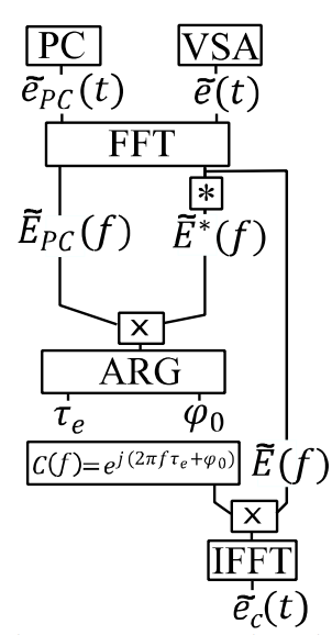
The slope of this phase is proportional to τe and the value of φ0 is defined as the value of the phase at the origin (centered on 0 in complex envelope). The synchronization is then carried out in the frequency domain by the multiplication by the coefficient C (f) thus obtained.

- Power Correlation Threshold : As a power notch (multi-carrier signal case), can lead to linear regression error, the algorithm allows to define a power threshold to eliminate all the cross correlation power which are below this level. Deleting these too small sample powers, the linear regression will fit the real phase slope and not an artifact. This parameter is useally optimize in multi-carrier signal case.
- Span-correlation : this parameter allows to define the span used to analyze cross-correlation function. Default value is 70% in order to delete the VSA analysis filter rejection effect.
- Time Domain:This time domain algorithm is based on
time cross-correlation coarse analysis, combined with
sub-sampling iterative optimization. It's recommanded for
multi-carrier signal.
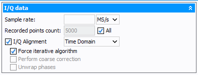
The determination of delay is based on find the sample location corresponding to the peak of the cross-correlation function. This provide a coarse correction (+/- 1 sample), then the peak of the cross-correlation function is interpolated to find the sub-sample delay.- Force iterative algorithm: This algorithm iteratively determines the crosscorrelation, predicts the peak location between sample, time-shifts and repeats. Less accurate at high signal-to-noise ratio and slower as the standard algorithm, but should always converge, even if "the" delay between two signals is not well- defined because of group delay variations, multiple periods etc.
- Perform coarse correction: perform a coarse correction (+/- 1 sample) using crosscorrelation between measured signal and reference signal. The location of the peak of the cross correlation function denotes the delay, with a resolution of one sample.
- Unwrap phase: removes phase jumps in excess of PI in positive and negative direction.
- Frequency Domain:This time domain algorithm is
based on frequency cross-correlation analysis. It's recommanded
for single carrier signal because it provide the best trade-off
between accurary and measurment time cost.
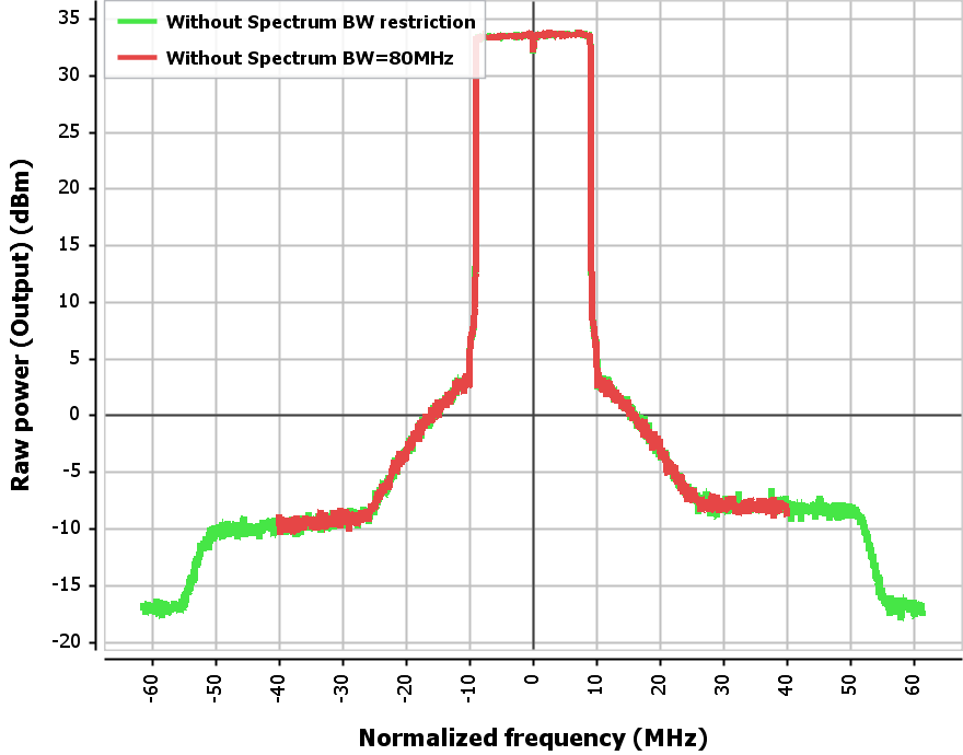
Spectrum
Spectrum setting allows to define an arbitrary spectrum span. This can be used to delete VSA filter effect.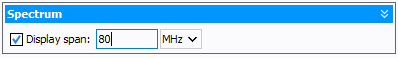
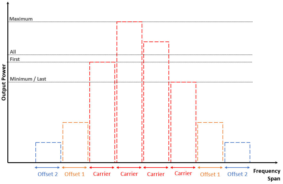
Adjacent Channel Power Ratio (ACPR)
 to add one or multiple lines
in the Carrier Settings (Main channels = Reference channels) or Offset Settings
(Adjacent or Alternate channels).
to add one or multiple lines
in the Carrier Settings (Main channels = Reference channels) or Offset Settings
(Adjacent or Alternate channels).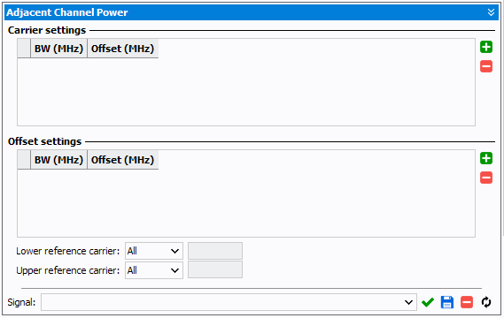
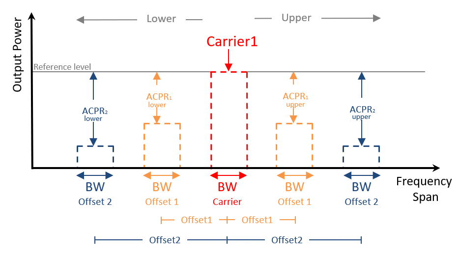
Lower and Upper reference carrier are used in the case of multi-carrier signals. There is serevals references :
- All : Mean power of all carriers
- Minimum : Minimum carriers power of all carriers
- Maximum : Minimum carriers power of all carriers
- First : First carriers power from left to right
- Last : Last carriers power from left to right
- Custom : Select the carrier you want to take as reference
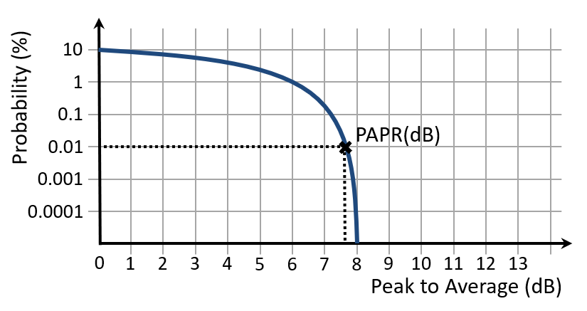
Complementary, cumulative Density Function (CCDF)
CCDF is a statistical distribution of the waveform power calculation performed in time domain. This measurement provides insight of instantaneous power as a function of time.

Dynamic AM/AM & AM/PM
The dynamic AM/AM & AM/PM measurements allow to record the instantaneous gain of the DUT over time.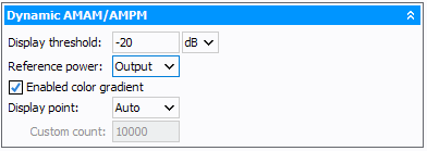
- Display threshold: limits the display over a defined power range.
- Reference Power: select the reference power between 'Input' and 'Output'. This reference power allows defininig which X-axis power is used to plot the Dynamic AM/AM & AM/PM
- Enabled color gradient: allows to apply gradient density coloration on AM/AM & AM/PM traces (can slow down measurement)
- Display point: Select "Auto", "All" or "Custom" to limit number of point displayed or improve display speed depending on the waveform size.
- Custom count: define the number of AMAM & AMPM points to display.
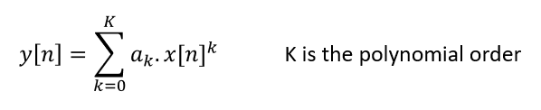
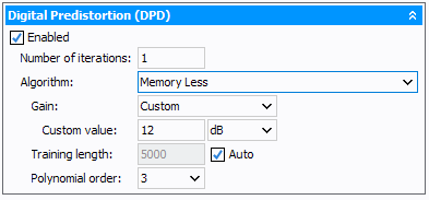
Digital Predistortion (DPD)
The digital pre-distortion measurement allows to evaluate the linearisability of the DUT.
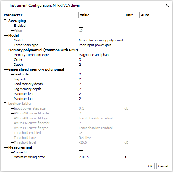
- Instrument: This option allows to used the intrinsic instrument DPD
capabilities, depends on the instrument used, therefore the measurement
options are related to the 'advanced options' of each Vector Signal Analyzerdriver. This measurement is only
available with the Ni PXI VSA for now.
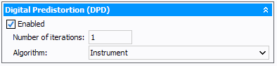
Number of iterations: sets the DPD iteration countAdvanced options: access Specific Digital pre-distortion (DPD) options in the driver (Model, Target gain type, model order…) which depends on the instrument used. Below, is an example of advanced options for Ni PXI VSA
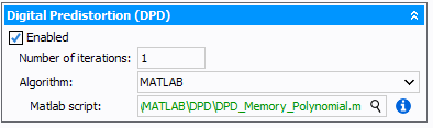
- Matlab: This option allows to used a custom matlab DPD algorithm. In
this case, IQSTAR will provide Iref & Qref from the reference signal
sent to the Vector Signal Generator (VSG) and Iout & Qout from the
Vector Signal Analyzer measurement. Custom matlab code will provide the
pre-distorted signal to IQSTAR, which will be automatically play. To learn
how to quick setup Matlab and IQSTAR see Getting Started: "Configure IQSTAR and Matlab environment to evaluate custom DPD algorithm".Note: Iref, Qref, Iin, Qin, Iout & Qout are corrected and time aligned before being sent to Matlab.
The matlab function has to respect the following syntax :
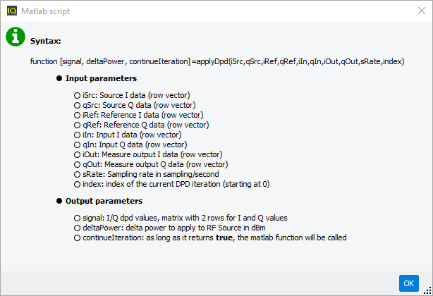
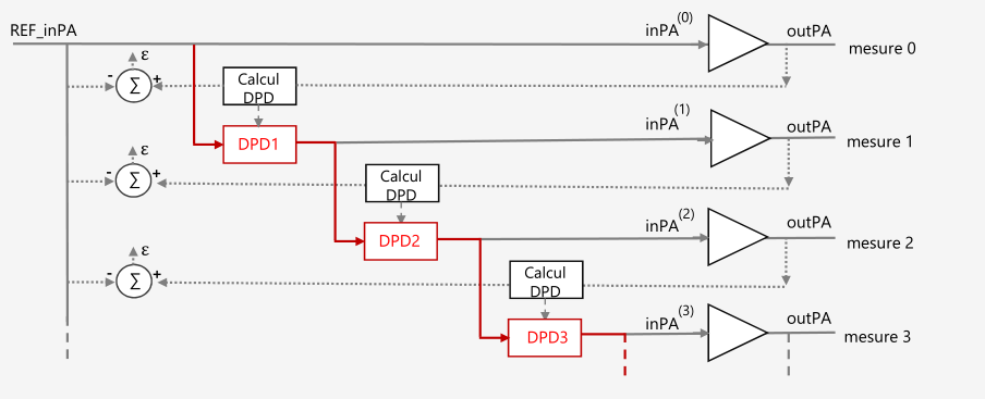
Input Parameters :- Iref & Qref : represent the IQ data of the reference signal corrected in DUT input plane
- Iin & Qin : represent the IQ data of the pre-distorted reference signal corrected in DUT input plane. For the first DPD iteration (index=0) Iin=Iref & Qin=Qref. Below is represented the DPD training sequence using multiple iteration.
- Iout & Qout : represent the IQ data measured with the VSA and time aligned with IQin & IQref and corrected in DUT ouput plane
- sRate: represent the IQ data sampling rate
- index: represent the actual iteration.
-
- Signal: represent pre-distorted signal that will be applied to evaluate DPD (matrix with 2 rows I & Q).
- DeltaPower: represent the back-off value to apply to the VSG in dBm.
- ContinueIteration: While it return True, Matlab function will be called. If returns False, number of iterations defined in IQSTAR will be take into account. This boolean allows to skip number of iterations defined in IQSTAR while it returns True. Through this boolean, the number of iterations can be handle in Matlab function rather than IQSTAR interface.
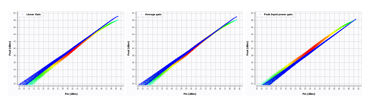
- Sample-based DPD: A key question during amplifier design is the
maximum performance of a device assuming perfect DPD. With the sampled-based
DPD approach, a given waveform is directly pre-distorted without any DPD
model. This approach can be use to evaluate and compare power amplifer
rather than to sort out the influences of different DPD model. This method
predistorts the input signal on a sample-by-sample basis. The sample based
approach, allows the modelling of any memory effect without increasing the
complexity, but increasing the number of DPD iteration. In this mode, IQ
averaging is mandatory to reduce noise impact.
 Note: Averaging option is available in "advanced driver option" as described below:
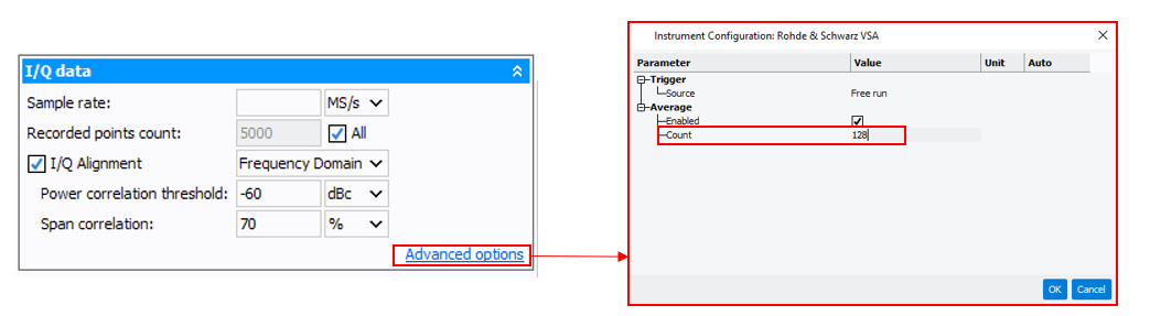
Gain : allows to choose the (Pre-distorter + DUT) final gain. Can be Average, Linear, Peak Input Power Gain or Custom.
- Memory Less: Using this DPD algorithm, a memory less presitorter will
be applied, as descirbed below:
Gain : allows to choose the (Pre-distorter + DUT) final gain. Can be Average, Linear, Peak Input Power Gain or Custom as described above.
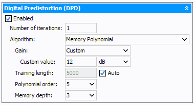
- Memory Polynomial: Using this DPD algorithm, a memory polynomial
presitorter will be applied, as descirbed below:

Gain : allows to choose the (Pre-distorter + DUT) final gain. Can be Average, Linear, Peak Input Power Gain or Custom as described above.Training Length: allows to select the number of sample used to extract pre-distorter model. "Auto" will adapt the best number of sample to reach the best trade-off between measurement speed and DPD accuracy.
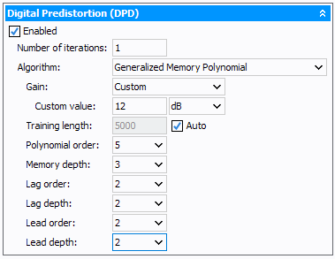
- Generalized Memory Polynomial: Using this DPD algorithm, a
generalized memory polynomial presitorter will be applied, as descirbed
below:
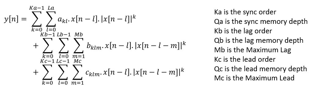
Gain : allows to choose the (Pre-distorter + DUT) final gain. Can be Average, Linear, Peak Input Power Gain or Custom as described above.Training Length: allows to select the number of sample used to extract pre-distorter model. "Auto" will adapt the best number of sample to reach the best trade-off between measurement speed and DPD accuracy.
- Nanosemi Single-Band: Allows to select "NanoSemi" DPD single band
algorithm. To learn how to install "NanoSemi" DPD, visit Getting Started : "NanoSemi integration in IQSTAR".
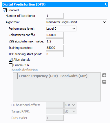
- DPD Level: Specifies the performance level of DPD algorithm
- rho: Specifies the robustness coefficient (0.0000001 to 1). Typical value is 0.1 for signal bandwidth of 60 MHz and above and 0.001 for signal bandwidth below 60MHz.
- VSG Absolute max value: Specifies the allowed growth, or headroom, in the waveform amplitude.
- Training samples: Specifies the number of samples to use when training the DPD (>32k samples and less than the number)
- TDD training start point: Specifies the DPD training algorithm such that the algorithm operates on input samples in the range
- Align signal: Allows to align signal.
- Nanosemi Dual-Band:Allows to select "NanoSemi" DPD dual band
algorithm. To learn how to install "NanoSemi" DPD, visit Getting Started : "NanoSemi integration in IQSTAR".
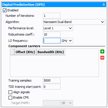
- Robustness coefficient: Specifies the robustness level. The value range is 1 to 10. The default value is 10, which is the most robust level.