
1-Tone Measurement Panel: Receiver
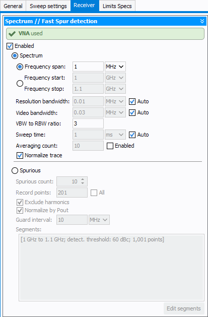
Once initialized, the green message will specify which one of the Supported RF Sources or of the Supported Vector Network Analyzers will be used to acquire the spectrum trace. This will be influenced by the "Give priority to the VNA for spectrum measurement" option.
Spectrum Mode:
- Frequency span / Frequency start & stop:used to choose the span
method, either by direct span definition, or by start and stop frequency
definition.Note: In "Frequency Span" mode, Spectrum center frequency is defined by the Fequency Sweep Settings defined in the 1-Tone Measurement Panel: Sweep Settings panel.Note: In "Frequency Span" mode, the span value can be set to zero, in order to work in "zero span" mode with the Spectrum. Therefore, the traces results will be in time domain in order analyze time domain pulse shape.Note: In "Frequency Start/Stop" mode, Spectrum frequencies settings are not correlated with the Fequency Sweep Settings defined in the 1-Tone Measurement Panel: Sweep Settings panel. This allows to analyze and store a constant frequency windows for each sweep conditions.
- Resolution bandwidth:Sets the VSA RBW to the defined value. If Auto is check, puts the RBW in auto mode.
- Video bandwidth:Sets the VSA VBW to the defined value. If Auto is check, puts the VBW in auto mode.
- VBW to RBW ratio:Sets the ratio between VBW and RBW, becomes unavailable if the RBW or VBW is manually set.
- Sweep time:Sets the VSA sweep time if specified, otherwise let the instrument run in automatic mode.
- Averaging count: Sets the number of averaging if enabled.
- Normalize trace: If set, the spectrum trace will be normalized to 0, otherwise, the data will be corrected in terms of power using calibrated measurement done by VNA or ouput power sensor.
Advanced Options : regarding of the intrument used (Supported Vector Signal Analyzers), allows to set more advanced parameters such as the IFBW filter, the trigger to use (free run, ext trigger input channel), attenuation and reference levels...). It is specific to the instrument used because of its capabilities.
Fast Spurious Detection Mode:
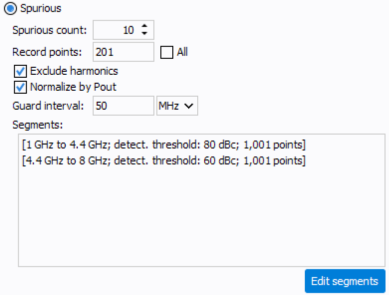
- Spurious count: Maximum number of spurious that can be saved in the output file. At the end of the meaurement, a corresponding number of data will be saved, named Spurious X [Frequency] and Spurious X [Power] where X goes from 1 to spurious count value. The current max possible value is 20 spurious.
- Record points: Number of final points to save as a spectrum trace. This number can be lower than the sum of all segments number of points. This will greatly improve the file size as the complete spectrum traces is saved for every measurement condition. Checking "All" will not rework the trace with the specified number of points.
- Exclude harmonics: If checked, the harmonics will not be taken as spurious frequencies.
- Normalize by Pout: If checked, the spectrum data will be normalized to Pout read at the DUT output plane.
- Guard interval: Sets an area of the span specified around the generated frequency and its harmonics where spurious cannot retained as such and are not registered.
- Segments:Table of the test description to run, click on Edit
segments to open the editor and change the configuration:
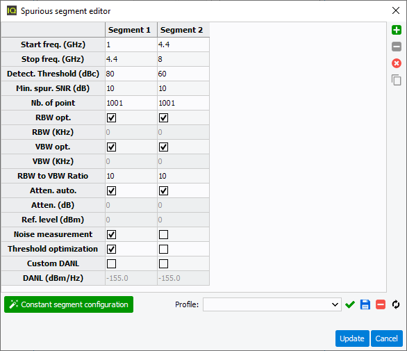
The center part of the editor is the table used to describe the segments to analyse. On the top right corner are the buttons to add one segment, remove one segment or remove all segments (from top to bottom).
Those segments are composed of multiple properties :
- Start frequency:start frequency of selected segment
- Stop frequency:stop frequency of selected segmentNote: Start frequency of next segment should be equal to stop frequency of the previous segment.
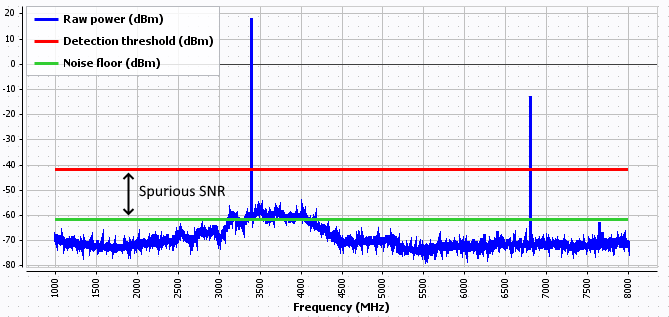
- Detection Threshold (dBc) : level relative to the carrier power. If a frequency point is found with a power level greater than the threshold (Threshold [dBm] = Power @carrier [dBm] - Detection Threshold [dB]), then it is retained as a spurious.
- Minimum spurious SNR (dB): Margin to take bellow the detection
threshold . Use to lower the noise floor, in order for the spurious to
be detected of this specified value above the trace noise floor. If this
setting is too low (for exemple 0), the Noise floor will equal the
detection threshold, and small noise peaks can lead to a spurious
detection.
- Number of point: Defines the number of points to acquire, if this number is too low, saying that the frequency resolution defined by the number of points in the segment is too low compared to the guardband, a warning will pop-up.
- RBW optimum: If checked, the RBW is calculated to be the highest possible (fastest measurement) while passing the specifications (minimum detectable spurious level, SNR). Otherwise, user specified RBW is used.
- RBW: Manual definition if optimization is disabled.
- VBW optimum: If checked, the VBW is equal to the RBW divided by the ratio specified. Otherwise, user specified VBW is used.
- VBW: Manual definition if optimization is disabled.
- RBW to VBW ratio: Ratio RBW/VBW
- Attenuation - Auto: If checked, uses the auto attenuation algorithme of the spectrum analyser, otherwise, sets the values defined.
- Attenuation (dB): Manual definition if optimization is disabled.
- Ref. level (dBm): Manual definition if optimization is disabled.
- Noise measurement: Allow the measurement of the noise floor trace
with those segment settings. If set, the spectrum will record a
supplement trace with the RF being off and the biasing being off. This
will allow to save the real noise floor with the specified settings, and
see the added DUT noise. This setting allow the observation of the DUT
noise. To measure this spectrum trace, a measurement is performed while
the DUT is biased, but without RF. This can result as in the example
bellow, where we can clearly see the working bandwidth of the PA (meant
to work up to 4.2GHz). This rejected noise measurement can be usefull to
see the PA contribution to the spectral noise.
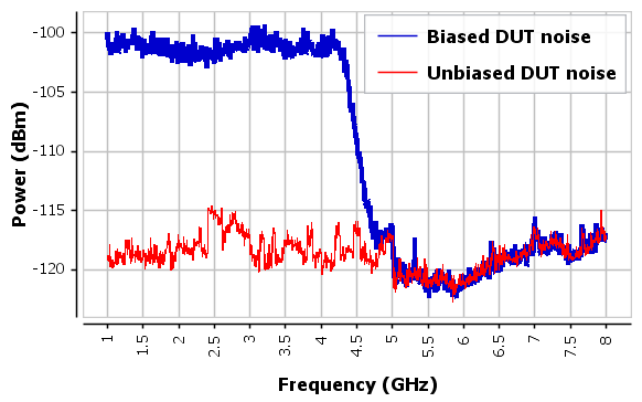
The above red trace will never be saved nor acquired as it represents the spectrum noise floor for a given RBW. The higher the RBW, the higher the noise floor will be, following the equation: Noise Floor = DNAL(1Hz) + 10 * log10(RBW). The blue noise trace will be acquired if this option is checked, and displayed in the graph. This trace will not be used to compute anything, it is simply in order to visualize the DUT spectral performances.
- Threshold optimization: Allows dynamic measurement analysis in
order to apply a correct RBW to have the lowest noise possible within
the specification. By selecting this option, multiple measurements will
be made for each segment, with one more measurement if the noise
measurement option is also checked. Here is the detail on a spurious
run, where only the first segment is set to this optimization:Note: This option will adapt the RBW so that the DUT generated noise matches the theorical VSA noise. The noise measurement option will acquire the DUT noise without this adaptative RBW algorithm, so the RBW will be set for the theorical noise floor excpectations, so before the optimization algorithm.
- The first measurement is made for the theorical RBW
calculated with each segment parameters. The needed RBW is
calculated following the output power, the detection
threshold, the SNR, and the attenuation level. In our case,
it is calculated to be 300KHz. We obtain this following
trace:
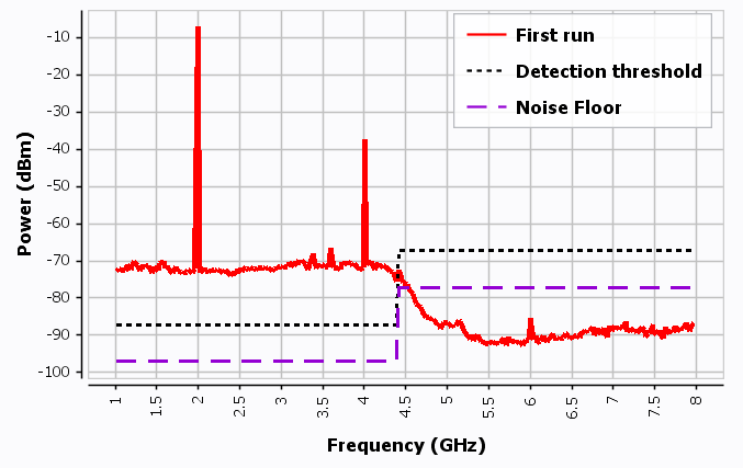
We can clearly see in this example that the first segment is influenced by the noise rejection of the PA, and so the theorical calculation (assuming no noise generation) is wrong. If it is unchanged, the frequencies above the detection threshold will be interpreted as spurious. On the second segment, the RBW was capped to the max possible RBW for the instrument and the trace is still under the thresholds, meaning that this RBW is compliant.
- The second measurement will analyze the first one and adapt
to look for some improvements. For this, for each segments,
the trace average will be calculated to deduce a potential
noise floor and recompute the RBW to be set at a lower
value.Note: In order for this algorithm to converge without incoherences, the segments must be defined with low spans, or the computed averages will not be representative of the frequency band noise.After some steps, the RBW is recomputed multiple times. In this case, the offset of roughly 20 dB between the noise floor and the first run trace was reduced in the new RBW calculation.
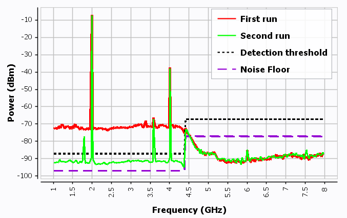
We can now see that this second run improved the trace noise, but not enough to be on the theorical, desired noise floor. On the other hand, the second segment did not change as the option was not checked. If it however would have been checked, the optimizer would have tried to increase the RBW in order to make the sweep faster, but would not have had any impact as it is already maxed out. - The third measurement is then performed with the applied
RBW. The trace segment average was compliant with the noise
level, so the optimization stopped. This finally ends up
with the last iteration with a RBW of 100Hz.
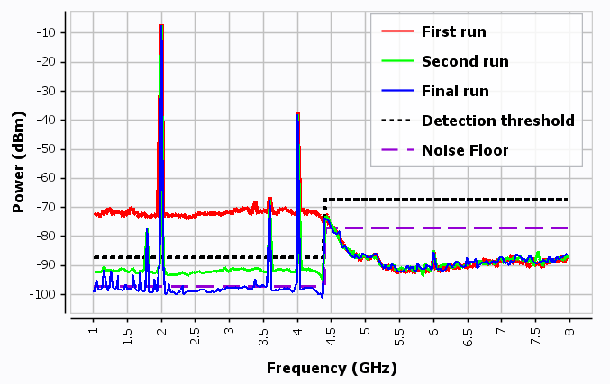
This final measurement adapted well the RBW to shift the trace noise around the theorical wanted noise floor. The major tradeoff is the requirement of multiple sweeps to adapt the RBW, slowing the measurement. However the main advantage is the automation of the sweep, specifically at low powers, where the DUT has an higher noise level than the noise floor of the VSA for a specific RBW.Note: The RBW is a discrete value, so the VSA might not surimpose perfectly the trace and the theorical noise.
- The first measurement is made for the theorical RBW
calculated with each segment parameters. The needed RBW is
calculated following the output power, the detection
threshold, the SNR, and the attenuation level. In our case,
it is calculated to be 300KHz. We obtain this following
trace:
- Custom DANL: if checked, allow the definition of a custom DANL value for the current segment. As this value is defined as one value, a user input is allowed to put a real, measured value of the DANL for the specific segment frequency range.
Bellow the table is the Segment configuration assistant, which is used to defined a lot of segments with the same properties.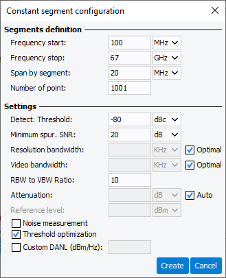 The settings are exactly the same as previously described. Hitting create will import the specified number of segments into the spurious editor where they can next be modified one by one if needed.Note: This assistant overwrite the current spurious configuration.It is also possible to load / save / remove / refresh profiles and so manage different segment configurations.
Once done with the configuration, hit Update to apply new settings, Cancel to go back without changing anything.
Related Information: