How to simulate a complete RF Chain thanks to accurate behavioral models ?
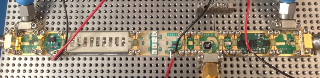
In this study, we have built a complete Down converter RF chain using some building blocks provided by X-Microwave. The aim was to anticipate the global performance of the system through an accurate system simulation.
For this purpose, a behavioral model was extracted for each circuit using VISION, our modeling and simulation tool. Finally, the different blocks were assembled to build a down-converter chain, both in the simulation, and with a real prototype.
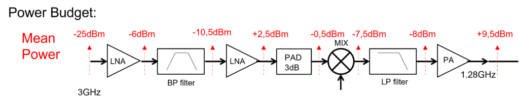
The very first step was to start with a top-down design approach. In our study case, the aim was to convert a 3GHz signal into a 1,28GHz signal with a 4,28GHz local oscillator. The input power of the signal is below -20dBm, and we wanted to obtain an output signal with a power higher than 9dBm.
According to these specifications, we decided to use the build the following subsystem.
After a quick survey, we have identified and supplied each building block. These circuits have been then measured individually.
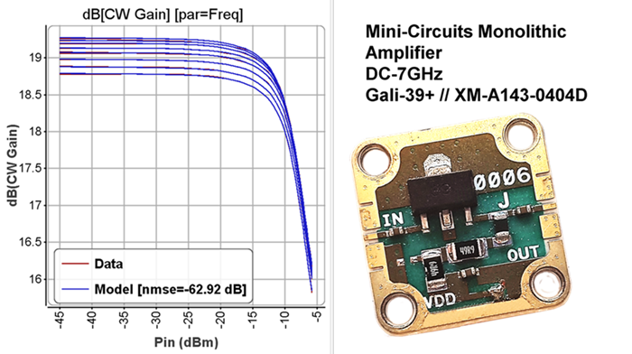
The first LNA had Gain of 19dBm, but with some dispersion according to the carrier frequency (f0). In our work, we named this dispersion “high frequency memory effects”, as it can create some distortion when a modulated signal is amplified, because of the gain variation in the bandwidth of interest.
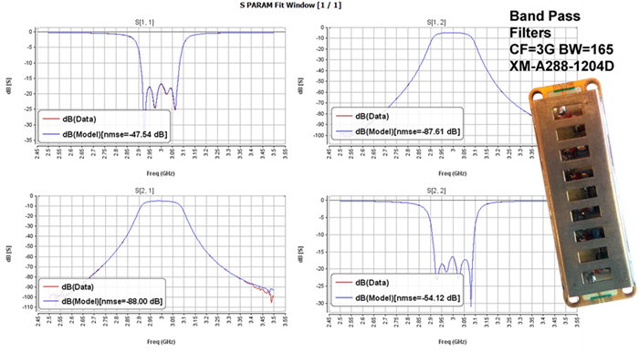
Regarding the filter, we measured the S-parameters. The aim of this bandpass filter was to eliminate all the signals expect the input signal within 200MHz around 3GHz. Our behavioral model reproduces the filter characteristic very well.
Note that the time domain simulator cannot just use one S-parameter touchtone file measured in the frequency domain. This is the reason why our model purpose is to reproduce this behavior, while enabling for time domain simulations. The same approach was used for all the passive circuits (low pass filter and attenuator)
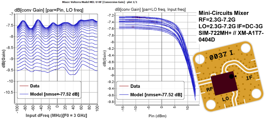
For the mixer characterization, we swept the input carrier frequency and the LO power to evaluate the nonlinear behavior of the frequency converter. We can observe that on top the nonlinear behavior, we also have some gain ripples depending on the input carrier frequency.
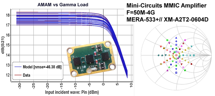
Finally, we measured the PA performances at different frequencies and power levels, for different load impedances using a load impedance tuner provided by Maury Microwave. In the graph below, the performances are displayed at 3GHz for different load impedances. We wanted the model to be valid for non-50 Ohms operating conditions because we knew that our down-converted could be loaded by some elements that would not be perfectly matched.
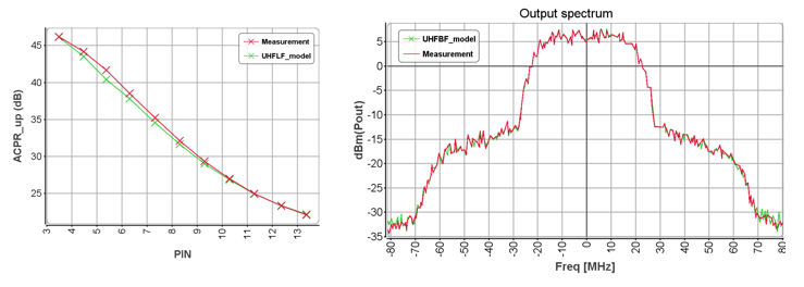
It was also important do validate the nonlinear behavior of the PA with modulated signals. In the graph below, we estimate the global performances with a 256QAM modulated signal, with an instantaneous bandwidth of 42MHz, with an input signal power swept between 3 and 13dBm to observe the spectral regrowth simulation capabilities. This simulation was done for a 50-Ohm load impedance, but the same can be provided for any impedance close to the pattern of load impedances used for the model extraction.
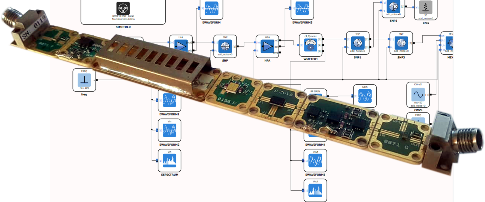
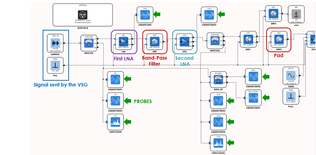
After extracting all these different circuits models, a simulation was performed for the complete down-converter assembly. We were then able to simulate the down-conversion function for different kinds of signals (one tone, two-tone, pulsed, modulated signals). The system architecture is represented in the diagram schematic below. Different signal probes enable to estimate the system performances between the different building blocs.
At the same time, we assembled all these circuits together, to get a complete measurement of the down-conversion chain, thanks to the building blocks provided by X-Microwave. This concept enables us to do a true performance comparisons, as the measurement and the simulation reference planes are the same in both cases. Indeed, measurement deembeeding is always a tedious job when the simulation results should be benchmarked.
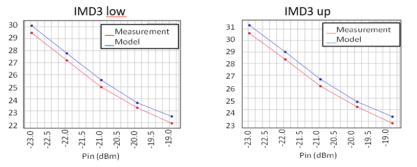
The comparison between the measurements and the simulation results of the overall subsystem were carried out for different stimuli, different powers and different impedances. As an example, below are some results for 2 tone signals, when the input power is swept from -23dBm to -19dBm with a two-one spacing of 60MHz.
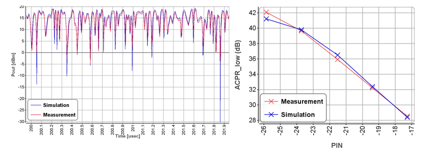
Time domain simulation enables to observe the data waveform for different power levels, such as 1dB of gain compression as shown below. Thanks to some FFT post processing, it is then easy to calculate the ACPR regrowth for different power levels.
This work was carried out thanks to measurement, modeling and simulation tools presented for the first time during the IMS conference during the ARFTG conference. “Wideband test bench dedicated to behavioral modeling of non-linear RF blocks with frequency transposition and memory” Published in : 2018 91st ARFTG Microwave Measurement Conference (ARFTG), DOI: 10.1109/ARFTG.2018.8423815
If you want to get more details on the technique used to measure, extract and simulate these models: