INTRODUCTION

The arrival of the 5G has considerably changed the design process of wireless communication systems. In this new generation, there is a need to improve the area throughput, but allocating more bandwidth (physically impractical) and deploying more base stations (high deployment cost, inter-cell interferences) is not feasible.

Therefore, new modulation and multiplexing techniques are necessary to improve the spectral efficiency per cell using the base stations (BSs) and bandwidth already in place. Beamforming in phase arrays and massive MIMO is used to improve the architecture’s performance.

Under these conditions, antenna designers face new challenges: theoretical beam steering is modified when connecting the antenna to the rest of the systems in the radio chain. Thus, a collaboration between designers in charge of each system becomes more relevant to achieving the expected overall performance, and a tool that all of them can use becomes necessary.

This white paper presents a new approach based on the simulation of accurate behavioral models to analyze undesired effects when connecting each system to improve beam steering.

PROBLEMATIC

Beamforming is the technique where antennas are controlled, either analog, digitally or hybrid analog-digital, to direct the signal to the user equipment (UE).

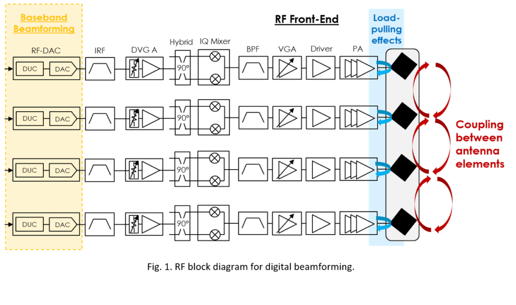
Digital beamforming (Fig. 1) is used to get full flexibility in the antenna radiation patter

However, digital beamforming faces a challenge in terms of power consumption and digital processing as the frequency increases. Therefore, for frequencies higher than 6 GHz (FR2), hybrid analog-digital beamforming (Fig. 2) becomes the most useful technique, where multiple beams can be created with the same power for all antennas and only one phase per signal.

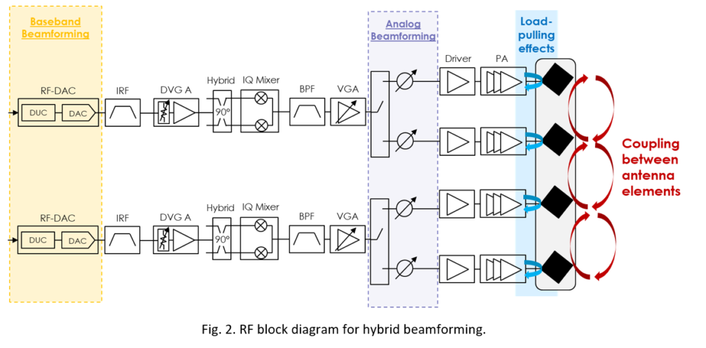
The antenna’s connection to the different systems of the chain introduces phase errors that may change the initial beam-steering angle. In the case of hybrid analog-digital beamforming, the presence of digital step attenuators (DSA) and digital phase shifters (DPS) used for the analog beamforming introduce losses that need to be considered at the design stage.

In addition, the connection of a PA at each port of the antenna introduces load-pulling effects that may degrade the PA behavior. Moreover, coupling effects between the antenna elements may reduce the antenna performance. Therefore, a tool enabling the analysis of these effects based on accurate behavioral models is necessary to improve beam steering.

BEHAVIORAL MODEL EXTRACTION

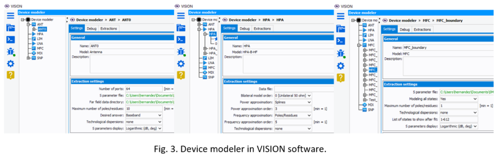
Behavioral models of the antenna, the PA and the DSA and DPS can be extracted using the device modeler of the VISION Software (Fig. 3).

In this example, using the EM-Link tool provided with VISION, the S-parameters of the antenna provided by HFSS from Ansys are converted into an equivalent behavioral model for bilateral data flow and transient simulations. Thus, all the coupling effects between the different patches of the antenna are known. Depending on the beam steering angle, these coupling effects will create a change of the active load provided to the RF Front-End.  The Power Amplifier behavioral models can be extracted from measurements, or Harmonic Balance circuit-level  simulation data, using tools such as ADS from Keysight or Microwave Office from Cadence. These different behavioral models can be then linked altogether using the system schematic editor.

This work compares results obtained using a PA behavioral model that considers load-pulling effects (B-HF) with a PA behavioral model that considers a circulator at the output of the PA (U-HF).

The DSA and DPS are identified in a multi-function-chip (MFC) model that accurately predicts their behavior while considerably reducing the measurement data necessary to extract it.

ACTIVE ANTENNA SIMULATION

The detection of errors at the antenna’s input and introduced by the systems in the radio chain is analyzed in simulation using the System Architect module of the VISION Software. First, the active antenna is simulated while considering digital beamforming through ideal sources.

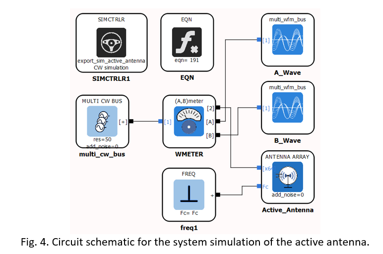
The antenna is a 4×8 dual-polarized active antenna in the band 3.4 GHz – 3.8 GHz with 64 ports. Bus blocks are used in VISION to connect a source at the input of each one of them. Fig. 4 shows the circuit schematic where beam steering is carried out through the phase of the ideal sources.

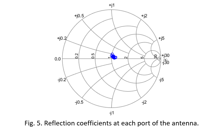
Probes have been connected to obtain the A and B waves at the input of the antenna enabling the calculation of different parameters such as the reflection coefficient at each port (Fig. 5)

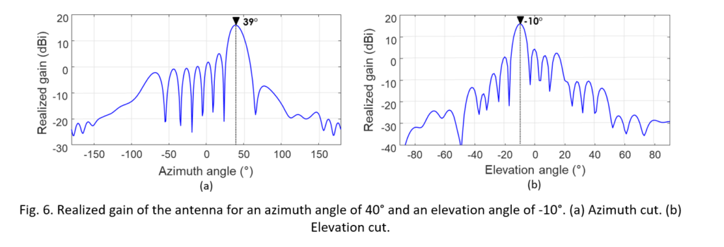
The radiation pattern can be calculated using the far-field data exported from an EM simulator from the A- and B-waves at the input of the antenna. Fig. 6 shows the antenna’s gain in the azimuth and elevation plans for an azimuth angle of 40° and an elevation angle of -10°. A deviation of 1° is observed in the azimuth cut associated with the antenna design.

SIMULATION OF THE PA (U-HF, B-HF) – ACTIVE ANTENNA CONNECTION

• U-HF : Unilateral Amplifier model which takes into account the High Frequency Memory effects
• B-HF :  Bilateral Amplifier model which takes into account the High Frequency Memory and the load impedance effects

Once the active antenna has been analyzed when connected to ideal sources, the behavioral model of a PA is connected at the input of each of its ports.

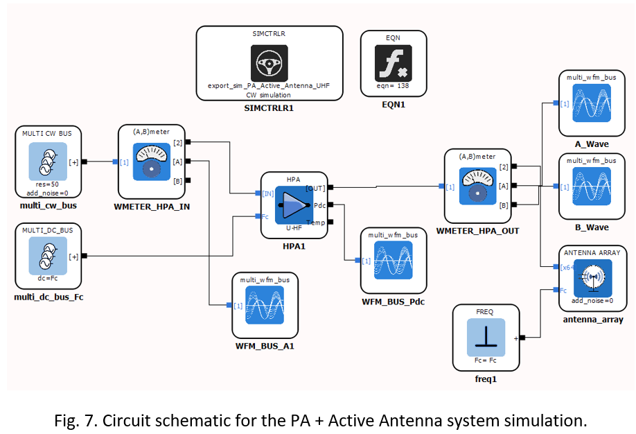
Two different behavioral models of the PA working at 3.6 GHz have been considered: a U-HF model (as if a circulator is connected at the output of each PA) and a B-HF model where load-pulling effects have been considered.

The effects of the PA’s connection at each port’s input are analyzed through the A- and B-waves, as well as the Pdc of the power amplifier (Fig. 7). Results from both models are compared.