Pole-Zero Identification Analysis
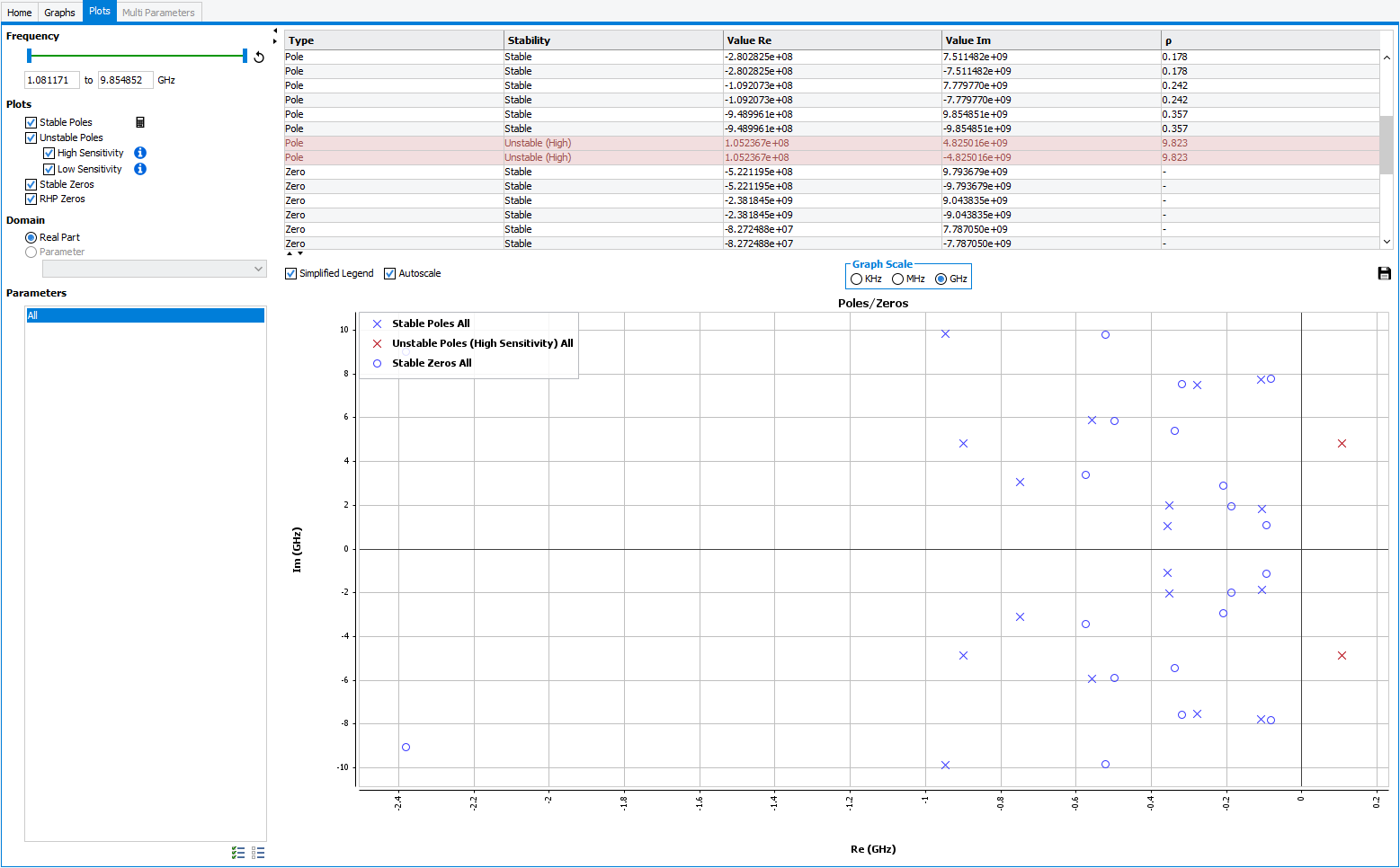
The pole-zero identification can be analyzed in detail using the Plots tab (Figure).
The frequency range can be modified thanks to the slider to see only the poles around a frequency of interest.
Plot menu with check box allow to choose what are the poles written in the table and plotted in the pole-zero map.
The values of the identified poles and zeros, as well as the ρfactor for the unstable poles (marked in color) are displayed on the table. The ρ factor for the stable poles can be calculated using the calculator: Calculate Sensitivity (ρ factor is only available for the SISO algorithm). Note that the frequency of the poles is given by the value of their imaginary part.
When using the SISO method, the unstable poles can be classified in three groups: high-sensitivity, low-sensitivity and very-low sensitivity poles. These three categories are given by the ρ factor extracted from the residue analysis:
- High-sensitivity poles, 1 < ρ (Unstable (High)): the circuit is unstable. Poles are colored in red in the table. For efficient circuit stabilization, consider introducing stabilization networks at those nodes or branches with a higher ρ value.
- Low-sensitivity poles, ρ <
1 (Unstable (Low)): poles may be physical (circuit
instabilities) or numerical (numerical noise with no effect on the circuit
dynamics). Further analyses are required: parametric or multi-node analyses for
verification. Note that poles with very low sensitivity (0.01 < ρ) are very
likely to be numerical.
Figure: STAN Tool Plots tab for a detailed analysis of the identification results with unstable poles colored in red in the table.