Perform statistical analysis

How to perform statistical analysis. Statistical analysis makes it possible to perform a simulation in which variables or models follow a statistical law.

To begin this task, you will need:

A licence of VISION System Architect. See Installation and licence setup.
To have opened a schematic. See Create or select a schematic
An extracted HPA-B-HF model in Device model. See Extract B-HF model

For example, we will analyze the responses of HPA-B-HF model to a load impedance whose value follows a specific statistical law. The basic steps to perform statistical analysis are:

Drag and drop the SIMCTRLR simulation controller block from the palette window in Simulation controls section to the schematic window.

Figure: Simulation controller block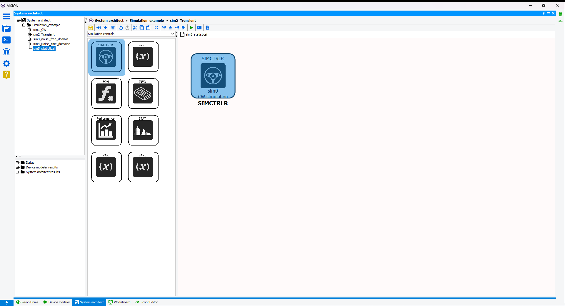
Double-click on the SIMCTRLR block to open the Parameters window. By default, the Simulation name is "sim0" and it is editable. Here we change the simulation name for "sim5_HPA_B_HF_noise_stat_analysis". In the Simulation mode tab, choose the Simulation mode by selecting CW simulation. Choose the Analyse type by selecting Statistical analysis. In the Solver tab, choose the Solver Type by selecting Algebraic solver I

Figure: Simulation mode
Drag and drop the VAR2 block from the palette window in Simulation controls section to the schematic window. Double-click on the VAR2 block to open the Parameters window. We sweep the input power thanks to variable "Pin_dBm" (sweep = 1) and we define the magnitude MAG and the phase PHI of the load impedance. The variable MAG will follow a normal distribution with the standard deviation σ = 0.04 and has 0 as expected value. The variable PHI will follow a uniform distribution in the interval -180° and +180°. For this, click on + to add a new variable. Insert the parameters as in the following figure and click on OK to create the variable then ok to confirm its creation in the VAR2 block. Repeate the same process for MAG and PHI variables.

Figure: VAR block
Now we will set up the schematic to simulate a HPA-B-HF model. Drag and drop the HPA block from the palette window in Non linear section to the schematic window. Double-click on the HPA block to open the Parameters window and fill in the Model parameter file field with the absolute or relative path of your extracted model in device modeler with the extension ".head".

Figure: HPA block
Drag and drop the CW-VS block from the palette window in Source section to the schematic window. Double-click on the CW-VS block to open the Parameters window and write "Pin_dBm" in the Amplitude parameter. Connect the CW-VS block output [+] with the input [in] of the HPA block.

Figure: CW-VS source block
Drag and drop the DC-VS block from the palette window in Source section to the schematic window. We will use this block to indicate the carrier frequency of the CW signal to the HPA block. Double-click on the DC-VS block to open the Parameters window, change the signal type to "real signal" and set the carrier frequency in DC value field. For this example, the carrier frequency is 1.28 GHz. Connect the DC-VS block output + with the input fc of the HPA block.

Figure: Set the carrier frequency
Drag and drop the 1-input ERHO block from the palette window in Linear lumped section to the schematic window. We will use this block to present specific load impedance at the output of the HPA block. Double-click on the ERHO block to open the Parameters window and set magnitude and phase of the reflection coefficient thanks to the MAG and PHI variables. Connect the HPA block output [out] with the input [+] of the ERHO block.

Figure: Present load impedance at the output of the HPA model
We will place a probe to measure the gain of the model. For the CW simulation, we need to use the RF Gain block. Drag and drop the RF Gain block from the palette window in Probe section to the schematic window:
- Connect the RF Gain block input [in] with the HPA block input [in].
- Connect the RF Gain block output [out] with the HPA block output [out].
Double-click on the RF Gain block to open the Parameters window and choose dB Magnitude and Phase as Gain type to display outputs db(gain) and phase(gain).
Figure: RF gain block
Statistical analysis allows us to observe the possible effects of the statistical variables on the figures of merit defined in the simulation. Here we are interested in the gain and power consumption. The block Performance monitor allows to analyze these figures of merit and we will see it after completing the simulation. Drag and drop the Performance monitor block from the palette window in Simulation controls section to the schematic window. Double-click on the Performance monitor block to open the Parameters window, set Waveform performance number parameter to 2 and edit the Waveform performances names parameter as Pdc and Gain. Connect the HPA block output pdc with the input pdc of the Performance monitor block. Connect the RF gain block output db(gain) with the input gain of the Performance monitor block.

Figure: Performance monitor block
Before performing the simulation, we will define the parameters of the statistical analysis thanks to STAT block. Drag and drop the STAT block from the palette window in Simulation controls section to the schematic window. Double-click on the STAT block to open the Parameters window and set the following parameters:
- Number of statistical trials: we will perform an input power sweep for 1000 load impedance values randomly drawn according to the statistical law defined in the VAR block.
- Statistical seed: set an integer value to initialize a pseudo-random number generator. By default, it's set to 0.
- Performance margin for yield calculation: the statistical analysis makes it possible to calculate the average of the quantities defined in Performance monitor block. We can thus calculate the number of trials where this quantity is close to the average with a margin defined in %. Here we set it to 2% of the average value.
- Number of bins for histogram calculation: After the statistical analysis, the histograms of the statistical variables defined in the VAR block and the quantities defined in the block are available. We set the number of bins to 20.
Figure: STAT block
The model can now be simulated. In the menu bar of the workspace window, click on Simulate>Run simulation or on the shortcut . The output console is displayed:

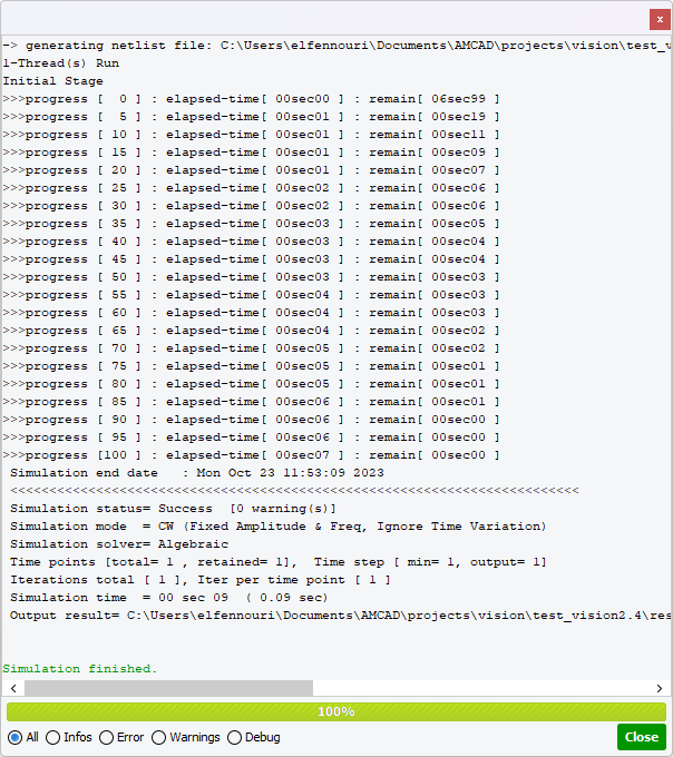
The console window contains the simulation time, the simulation mode, the repertory of the results, and also any warnings and errors encountered during the simulation.
When closing the console window, simulation results appear in the application tree in the folder named after the simulation "sim5_HPA_B_HF_stat_analysis". In Workspace window, the Log shows console information. Click on Output graphs tab to access the measurements provided by the probes. Select Waveform Perfs to display Pdc and Gain graphs. Pdc and Gain versus input power for all statistical trials on the load impedance value are displayed.

Figure: Waveform Perfs graphs

Click on Configure button to select a particular trial.
Figure: Waveform Perfs graphs - select a trial

Select Waveform Perfs Yield to display minimum, maximum and mean curves of Pdc and Gain. The Yield graph present the percentage of trials that respect the 2% margin defined in STAT block. We note that 100% of the trials respect the margin on the Pdc. In contrast, less than 80% of the trials are valid on the small signal gain. This decreases in gain compression.
Figure: Waveform Perfs Yield

Select Waveform Perfs Histogram to display the histogram of the MAG and PHI statistical variables and the simulation results of Pdc and Gain.
Figure: Waveform Perfs Histogram

Click on Configure button to select a particular value among the swept input powers.
Figure: Waveform Perfs Histogram - select a single value in swept parameter