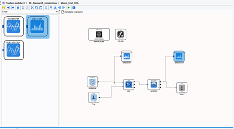
Perform 2-tone simulation

How to perform 2-tone simulation. 2-tone simulation in VISION allows to obtain time domain response of nonlinear circuit excited by 2-tone complex signal varying in frequency spacing and average power.

To begin this task, you will need:

A licence of VISION System Architect. See Installation and licence setup.
To have opened a schematic. See Create or select a schematic
An extracted U-HF-HPA model in Device model. See Extract U-HF model

The basic steps to perform a transient simulation are:

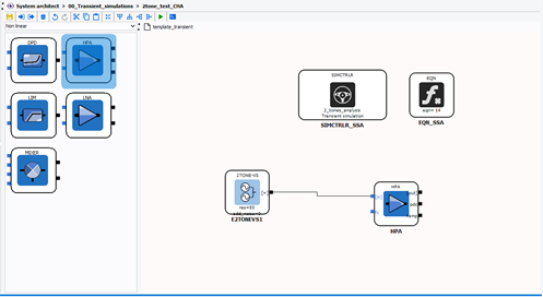
Drag and drop the SIMCTRLR simulation controller block from the palette window in Simulation controls section to the schematic window.

Figure: Simulation controller block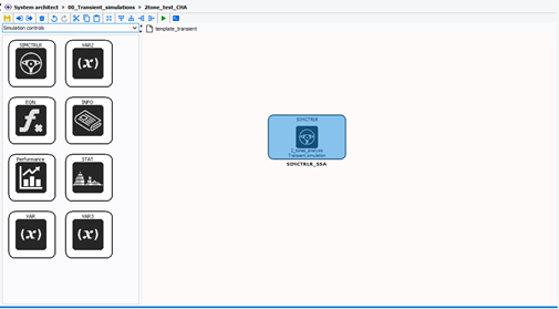
Double-click on the SIMCTRLR block to open the Parameters window. By default, the Simulation name is "sim0" and it is editable. In the Simulation mode tab, choose the Simulation mode by selecting Transient simulation. We will use two variables to fill the Final integration time, in seconds, and the number of time points. We will describe in the next step how to set up these variables. Choose the Analyse type by selecting Sweep analysis. In the Solver tab, choose the Solver Type by selecting Data Flow Solver
Drag and drop the EQN equation block from the palette window in Simulation section to the schematic window. Double-click on the EQN block to open the Parameters window. We create several parameters:

T_longest_memory = 1.57895E-08 ;

freq_BB_max = 200e6 ;

period_min = 1/freq_BB_max ;

nb_integ_period_min = 2*T_longest_memory/period_min ;

nb_integ_period_tran = (nb_integ_period_min-10) ? nb_integ_period_min:10 ;

nb_integ_period_ss=10 ;

nb_integ_period = nb_integ_period_ss;

freq_BB = spacing*1e6 ;

period_BB = 1/freq_BB ;

nb_sample_per_period = 40 ;

Tstop = nb_integ_period*period_BB ;

nb_sample = nb_integ_period*nb_sample_per_period ;

eps = freq_BB/2 ;

FREQ = 3e9 ;

These parameters are related to the 2 tones signal that we will use in this simulation.

T_longest_memory parameters : given by the device modeler log window when extracting the model as following:

Info: Estimated PA in-band memory duration is >= 6.66667E-09 sec
Figure: Log window after model extraction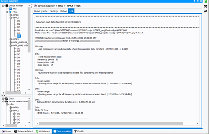

freq_BB_max : the maximum spacing between the 2 tones

FREQ = 8.2e9 : the center frequency between the 2 tones.
Figure: Equation block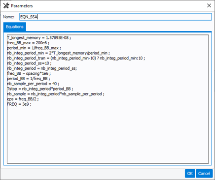
4Double-click on the SIMCTRLR block to open the Parameters window et write the equations in the following parameters:
- Final integration time: Tstop
- Number of time points: nb_sample+1
5. Now we will set up the schematic to simulate a HPA-U-HF model. Drag and drop the HPA block from the palette window in Non linear section to the schematic window. Double-click on the HPA block to open the Parameters window and fill in the Model parameter file field with the absolute or relative path of your extracted model in device modeler with the extension ".head".

Figure: HPA block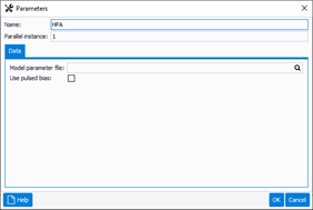
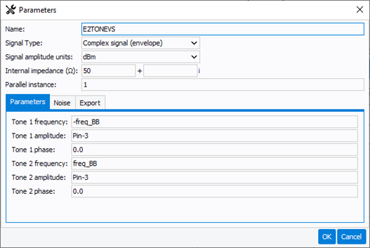
6. Drag and drop the 2-tones generator block from the palette window in Source section to the schematic window. Double-click on the E2TONESVS block to open the Parameters window. Fill in the Model parameter with freq_BB and Pin parameters as shown below. Connect the E2TONES-VS block output [+] with the input [in] of the HPA block.
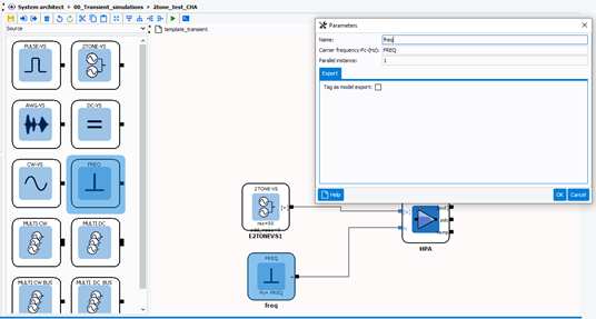
Drag and drop the DC-VS block from the palette window in Source section to the schematic window. We will use this block to indicate the carrier frequency of the CW signal to the HPA block. Double-click on the DC-VS block to open the Parameters window, change the signal type to "real signal" and set the carrier frequency in DC value field. For this example, the carrier frequency is 3 GHz. Connect the DC-VS block output + with the input fc of the HPA block.
Drag and drop the RES block from the palette window in Linear lumped section to the schematic window. We will use this block to present a 50 Ohms load at the output of the HPA block. Double-click on the RES block to open the Parameters window and set the resistance to 50 Ohms. Connect the HPA block output [out] with the input [+] of the RES block.
We will now place probes and scopes to measure spectrum, waveform and adjacent channel power ratio (ACPR). In a transient simulation, we use the W-meter block. Drag and drop two W-meter blocks from the palette window in Probe section to the schematic window:
- Place the W-meter between the HPA block and the RES block.
- Connect the HPA block output [out] with the W-meter block input [1].
- • Connect the W-meter block output [2] with the RES block input [+].
The W-meter block allows to measure incident and reflected power waves, respectively A and B. Double-click on the W-meter block to open the Parameters window and choose Incident & Reflected power wave (A-B) as Probe type.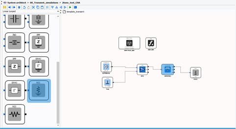
To measure the input and output spectrum, drag and drop the Spectrum block from the palette window in Scope section to the schematic window. Double-click on the Spectrum block to open the Parameters window:
- Place a first spectrum connected to the HPA input.
- Edit the Probe name to " Voltage_spectrum_input"
- Place a second spectrum connected to the [A] output of the W-meter.
- Edit the Probe name to " Voltage_spectrum_output"
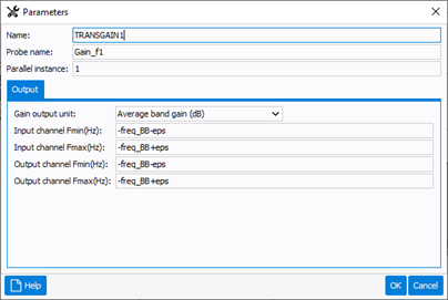
To measure the input/output gain at each 2 tones frequencies, drag and drop the TRANS_GAIN block from the palette window in Probe section to the schematic window.
- Place a first trans_gain connected to the HPA input and output.
- Edit the Probe name to " Gain_f1"
- Fill fields of each parameters as follow:
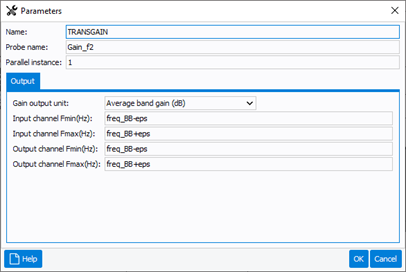
- Place a second trans_gain bloc connected to the HPA input and output.
- Edit the Probe name to " Gain_f2"
- Fill fields of each parameters as follow :
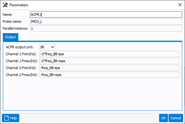
To measure the output IMD3 and IMD5 versus power and frequency spacing varaition, drag and drop the ACPR block from the palette window in Probe section to the schematic window.
- Place a first ACPR connected to the [A] output of the W-meter.
- Edit the Probe name to " IMD3_L"
- Fill fields of each parameters as follow:
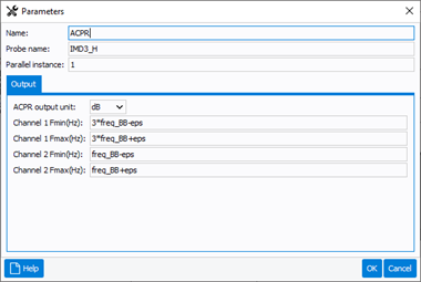
- Place a second ACPR connected to the [A] output of the W-meter.
- Edit the Probe name to " IMD3_H"
- Fill fields of each parameters as follow:
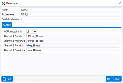
- Place a third ACPR connected to the [A] output of the W-meter.
- Edit the Probe name to " IMD5_L"
- Fill fields of each parameters as follow:
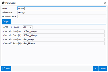
- Place a third ACPR connected to the [A] output of the W-meter.
- Edit the Probe name to " IMD5_L"
- Fill fields of each parameters as follow:
The differents probes are now define in order to probes the following spectrum :
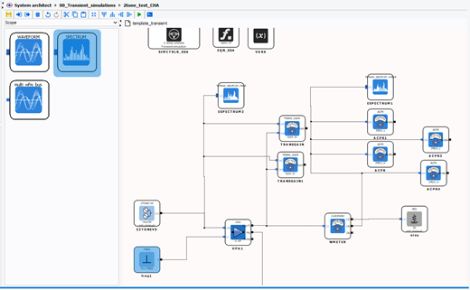
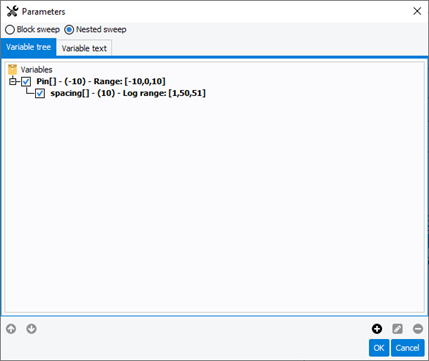
Last step is to define the frequencies spacing and power sweep. Double-click on the VAR block to open the Parameters window. We will set up two nested loops: the first one varies the power of the input signal "Pin_dBm" (sweep = 1) and the second the carrier spacing frequency "spacing" (sweep = 2). The syntax is as follows:
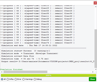
Double-click on the SIMCTRLR block to open the Parameters window and edit a name to the simulation. Here we change the name for "2 tones analysis”. The model can now be simulated. In the menu bar of the workspace window, click on Simulate>Run simulation or on the shortcut . The output console is displayed:
When closing the console window, simulation results appear in the application tree in the folder named after the simulation "2_tones _analysis". In Workspace window, the Log shows console information. Click on Output graphs tab to access the measurements provided by the probes. Click on Spectrum Probes in Figures section to display the input and output spectrum.

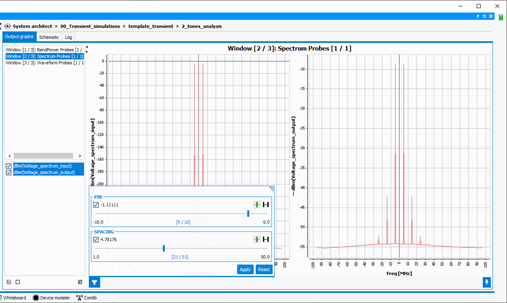
Filter can be use in order to plot spectrum for particular range of frequency spacing and power.
We can analyze the IMD3 and IMD5 results. Click on Output graphs tab to access the measurements provided by the probes IMD3_L, IMD3_H, IMD5_L, IMD5_H.

Some memory effects are highlighted with the variation of the IMDn level on the analysis bandwidth.