How to extract Bilateral High and Low Frequency memory (B-HFLF) model for High Power
Amplifier (HPA). The HPA-B-HFLF model is the most complete biilateral amplifier model. It
brings together the strengths of HPA-U-HFLF and HPA-B-HF models and eliminates their
limitations. This model makes it possible to represent quite faithfully both long-term
memory effects (polarization, thermal, trap) and short-term memory effects. This model is
therefore suitable for almost all applications (narrowband, wideband, variable envelope,
radar). On the other hand, it makes it possible to take into account the changes in load and
source impedance. .
Input files build from measurement or circuit simulation. Example data files
can be found in "data_example" folder in VISION installation directory.
The basic steps for extract an B-HFLF model are:
Create a new HPA device
In an opened project, you can create a device from Applications window
or Workspace window.
Figure: VISION window
From Applications window, right-click on Device modeler
and click on Create device. You can also right-click on
HPA and click on Create HPA device.
From Workspace window, click on Device modeler button,
select HPA and click on Open button then New
button.
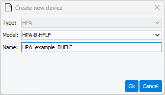
The Create a new device dialog box is displayed. Figure: Create a new HPA device
In Type field, select HPA.
In Model field, select HPA-B-HFLF.
In Name field, edit the name of your device. Here, we will name
it "HPA_example3".
Click on Create button to display the new device in the tree of
Applications window and the settings of the extraction in
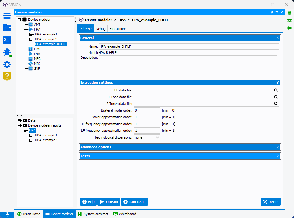
Workspace window.Figure: Extraction settings
Choose your data file
In the Extraction
Settings section, fill in the BHF data file field with the
absolute or relative path of your load-pull measurement or simulation file with
the extension .dat, .cst, .imx or .txt. In addition, fill in the 1-Tone data
file field with the absolute or relative path of your 1-Tone CW
measurement or simulation file with the extension .dat. Click on Browser button to open the file browser and select your file in the local
file system. The file browser opens directly to the data directory specified
when creating the project. Also, fill in the 2-Tones data file field with
the absolute or relative path of your 2-Tones simulation file or 3-Tones
measurement file with the extension .dat.
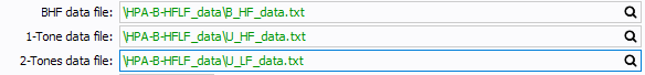
Tune power and frequency approximation order parameters
Figure: Model parametersIn Bilateral model order parameter, choose the order corresponding
to the measurement data.
In Power approximation order, HF frequency approximation order
and LF frequency approximation order fields, start to put low orders and
checks results graphically after extraction.
Nota Bene:
Bilateral part of the model is identified from the
CW load-pull measurement. This roughly corresponds to applying the principle
of extracting the HPA-U-HF model on several load impedances. The HPA-B-HF
model is declined in several bilateral order, ranging from 0 to 3.
The greater the order, the more the model is able to take into account
strong load mismatches in the nonlinear operating zone. It takes a minimum
of 3 load impedances to be able to identify the simplest bilateral model
(Bilateral order 1), 6 impedances for bilateral order 2 and 10 impedances
for bilateral order 3.
The power approximation order can not be
greater than the number of power points included in the data file.
The frequency approximation order can not be greater than the
number of frequency points included in the data file. If exceeded, VISION
will send a message in the Output Console window and automatically
truncate the order of approximation to the maximum number
allowed.
Also, you must take care to consider the frequency
approximation order as low as possible (do not seek a perfect fit of
the frequency characteristics by pushing the order of approximation to the
maximum).
The Technological dispersions option allows to
specify a distribution law of the gain (module) and phase shift
characteristics of the amplifier. Two laws of dispersion are possible
(Uniform or Gaussian law). The dispersion is characterized by two
parameters: the standard deviation Module, given in % of the nominal
value for the gain, and the standard deviation Phase in degrees for
the phase shift.
Extract behavioral model and check with output graphs
Click on Extract button to start the extraction
process of the model. The output console is displayed:
The message Model Fit Error is showing the normalized mean square error
(NMSE) between data and model. The output console also displays tips on
filters to apply to measurement data to improve model accuracy. Close the window
to see in the Applications window the number of the newly created
extraction, here, 001. The results are saved and can visualized at any time by
designating in the tree the associated extraction. Click on the Output
graphs tab to see comparisons between data and model. Figure: Output graphs after B-HFLF model extraction 001
Various graphs are available to check the quality of the model according
to three dimensions: power, frequency and load impedance.
To examine the quality of the approximation of the nonlinear pseudo
parameter S21, select Volterra Model HPA-B-HF [Output reflected power
wave: B2] in Figures section and choose graphs you want to
display in Graphs section:
Tick dB[S21 = B2/A1] [par=Pin, Load] to display, for different
input power and load impedances, the modulus of the nonlinear pseudo
parameter S21 in dB as a function of dFreq, the offset
between the central frequency of the device characterization band and
the frequency of the CW signal.
Tick phase[S21 = B2/A1] [par=Pin, Load] to display, for different
input power and load impedances, the phase of the nonlinear pseudo
parameter S21 in dB as a function of dFreq, the offset
between the center frequency of the device characterization band and the
frequency of the CW signal.
Tick dB[S21 = B2/A1] [par=Freq, Load] to display, for different
carrier frequencies and load impedances, the modulus of the nonlinear
pseudo parameter S21 in dB as a function of Pin, the
power of the CW input signal.
Tick phase[S21 = B2/A1] [par=Freq, Load] to display, for
different carrier frequencies and load impedances, the phase of the
nonlinear pseudo parameter S21 in dB as a function of
Pin, the power of the CW input signal.
To examine the quality of the approximation on the gain, select Volterra
Model HPA-U-HFLF [1Tone RF Gain] in Figures section and choose
graphs you want to display in Graphs section:
Tick dB[1Tone CW Gain] [par=Pin] to display, for different input
power, the modulus of gain in dB as a function of dFreq, the
offset between the central frequency of the device characterization band
and the frequency of the CW signal.
Tick phase[1Tone CW Gain] [par=Pin] to display, for different
input power, the phase of gain in dB as a function of dFreq, the
offset between the center frequency of the device characterization band
and the frequency of the CW signal.
Tick dB[1Tone CW Gain] [par=Freq] to display, for different
frequencies, the modulus of gain in dB as a function of Pin, the
power of the CW input signal.
Tick phase[1Tone CW Gain] [par=Freq] to display, for different
frequencies, the phase of gain in dB as a function of Pin, the
power of the CW input signal.
The graphs show the curves of data (from measurement or simulation) in red
lines and the extracted model in blue lines. The legend recalls the error NMSE
between model and data. If the number of curves makes the graphs unreadable,
click on Configure button to reduce the density of curves and/or limit the input
power range and frequency band. Select Volterra Model HPA-U-HFLF [2Tone RF/RF
Parametric Gain] in Figures section to display the parametric
gain between the input and output small-amplitude tone CW signal, depending on
input power and frequency. Select Volterra Model HPA-U-HFLF [2Tone RF/IMD3
Conversion Gain] in Figures section to display the conversion
gain between the input small-amplitude tone CW signal and the generated IM3,
depending on input power and frequency. Select Volterra Model HPA-U-HFLF
[1Tone DC consumption] in Figures section to display power
consumption of the device under 1-tone CW signal depending on input power and
frequency. Select Volterra Model HPA-U-HFLF [2Tone RF/DC Conversion Gain]
in Figures section to display conversion gain between the input
small-amplitude tone CW signal and the DC signal depending on input power and
frequency.
Check measurement aberration and noise measurement
The first extraction is an opportunity to verify the data. It should be noted
that 2-tone measurements may contain errors and numerical aberrations that may
make the identification of the model difficult and impoverish the final
precision of the model. VISION provides some tools to limit or eliminate these
phenomena in order to avoid doing measurements again. In Applications
window, click on your device, here HPA_example_BHFLF, to show up
Settings tab in the Workspace window. Click on Extraction
Options section to reveal some options:
Measurement aberration and noise polish filters: for the U-HFLF
model, the option CW power gain aberrations is available to
filter the noise that can be encountered on the 1-tone measurement data.
This options allows to approximate CW power gain curve with a polynomial
of order 1 or 2. The option Low frequency offset conversion gain
assure no long-term memory for close frequency tones by applying a smart
filter. The option Small signal conversion gain assure no
long-term memory for small signal input with a smart filter selection.
The user must choose the filter order appropriately.
Extraction power and frequency range tune: depending on the needs
or observations on the data, one can modify the range of input power
and/or the frequency band of the data with which the extraction of the
model can be performed.
The option
Frequency grid oversampling increases the frequency step in order to
improve the approximation of the phase, especially if this one presents a
variation greater than in radian according to the frequency.
Tune power and frequency range
If the first extraction is not satisfactory, it is necessary to increase the
order of approximation power and/or frequency taking into account the advice
displayed in the output console on the BF frequency approximation order and the
filters to be applied.
Apply a test plan
It is recommended to perform basic simulations after an extraction to check
the behavior of the model in the face of signals different from those used for
its identification. VISION provides tools to simply configure signals and
perform simulations directly after model extraction. In Applications
window, click on your device, here HPA_example_BHFLF, to show up
Settings tab in the Workspace window. Click on Test
plan section to reveal two options:
Automatic tests: this option allows you to perform simulations
with 2-tone and pulse signals whose settings are set automatically,
except for the pulse width period.
Normal test: this option allows simulations with CW, 2-tone,
pulse and white noise signals. You can also provide your own IQ file by
specifying the path of the file. (see Figure 8)


 Browser button to open the file browser and select your file in the local
file system. The file browser opens directly to the data directory specified
when creating the project. Also, fill in the 2-Tones data file field with
the absolute or relative path of your 2-Tones simulation file or 3-Tones
measurement file with the extension .dat.
Browser button to open the file browser and select your file in the local
file system. The file browser opens directly to the data directory specified
when creating the project. Also, fill in the 2-Tones data file field with
the absolute or relative path of your 2-Tones simulation file or 3-Tones
measurement file with the extension .dat.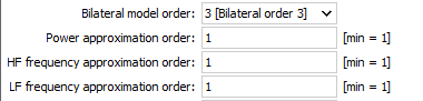 In Power approximation order, HF frequency approximation order and LF frequency approximation order fields, start to put low orders and checks results graphically after extraction.Nota Bene:
 Extract button to start the extraction
process of the model. The output console is displayed:
Extract button to start the extraction
process of the model. The output console is displayed: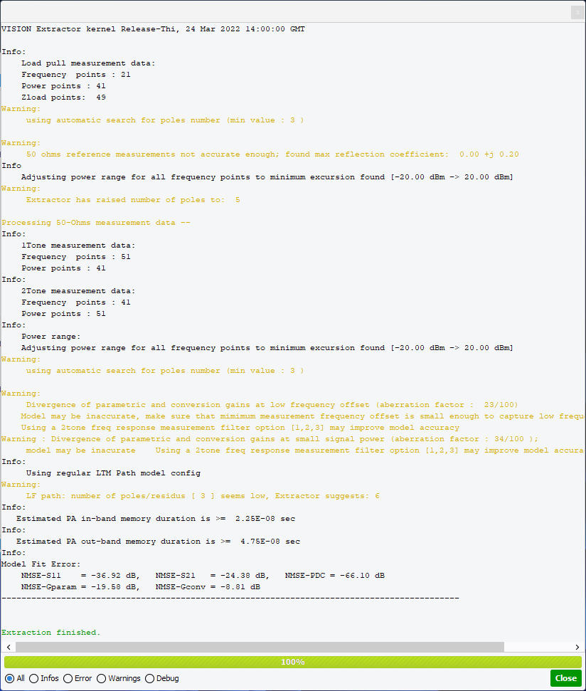 The message Model Fit Error is showing the normalized mean square error (NMSE) between data and model. The output console also displays tips on filters to apply to measurement data to improve model accuracy. Close the window to see in the Applications window the number of the newly created extraction, here, 001. The results are saved and can visualized at any time by designating in the tree the associated extraction. Click on the Output graphs tab to see comparisons between data and model.
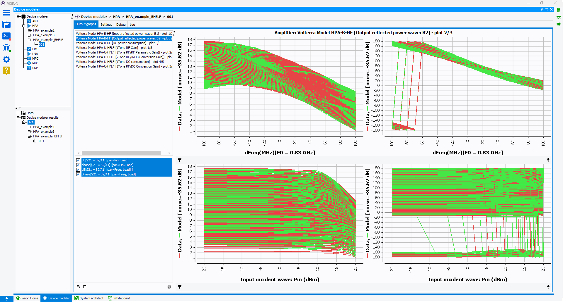
 Configure button to reduce the density of curves and/or limit the input
power range and frequency band. Select Volterra Model HPA-U-HFLF [2Tone RF/RF
Parametric Gain] in Figures section to display the parametric
gain between the input and output small-amplitude tone CW signal, depending on
input power and frequency. Select Volterra Model HPA-U-HFLF [2Tone RF/IMD3
Conversion Gain] in Figures section to display the conversion
gain between the input small-amplitude tone CW signal and the generated IM3,
depending on input power and frequency. Select Volterra Model HPA-U-HFLF
[1Tone DC consumption] in Figures section to display power
consumption of the device under 1-tone CW signal depending on input power and
frequency. Select Volterra Model HPA-U-HFLF [2Tone RF/DC Conversion Gain]
in Figures section to display conversion gain between the input
small-amplitude tone CW signal and the DC signal depending on input power and
frequency.
Configure button to reduce the density of curves and/or limit the input
power range and frequency band. Select Volterra Model HPA-U-HFLF [2Tone RF/RF
Parametric Gain] in Figures section to display the parametric
gain between the input and output small-amplitude tone CW signal, depending on
input power and frequency. Select Volterra Model HPA-U-HFLF [2Tone RF/IMD3
Conversion Gain] in Figures section to display the conversion
gain between the input small-amplitude tone CW signal and the generated IM3,
depending on input power and frequency. Select Volterra Model HPA-U-HFLF
[1Tone DC consumption] in Figures section to display power
consumption of the device under 1-tone CW signal depending on input power and
frequency. Select Volterra Model HPA-U-HFLF [2Tone RF/DC Conversion Gain]
in Figures section to display conversion gain between the input
small-amplitude tone CW signal and the DC signal depending on input power and
frequency.