How to extract Unilateral High Frequency memory (U-HF) model for Mixer (MIX). The
MIX-U-HF model is the simplest nonlinear mixer model. Extracting this model requires little
information about the component, i.e. 1-tone CW measurements, performed on a nominal load
impedance. It therefore takes into account only the dispersive effects present in the
operating band of the mixer and ignores other memory effects such as those due to
polarization or heating. It is a fixed LO signal model. Only the LO frequency variations are
taken into
account.
This model does not take into account load impedance changes.
An input file build from U-HF mixer measurement data or U-HF simulation
data. See "U-HF mixer scalar measurement" or "Simulation template for U-HF
Mixer data".
The basic steps for extract an U-HF model are:
Create a new Mixer device
In an opened project, you can create a device from Applications window
or Workspace window.
From Applications window, right-click on Device modeler
and click on Create device. You can also right-click on
MIX and click on Create MIX device.
From Workspace window, click on Device modeler button,
select MIX and click on Open button then New
button.
The Create a new device dialog box is displayed. Figure: Create a new mixer device
In Type field, select MIX.
In Model field, select MIX-U-HF.
In Name field, edit the name of your device. Here, we will name
it "MIX_example4".
Click on Create button to display the new device in the tree of
Applications window and the settings of the extraction in
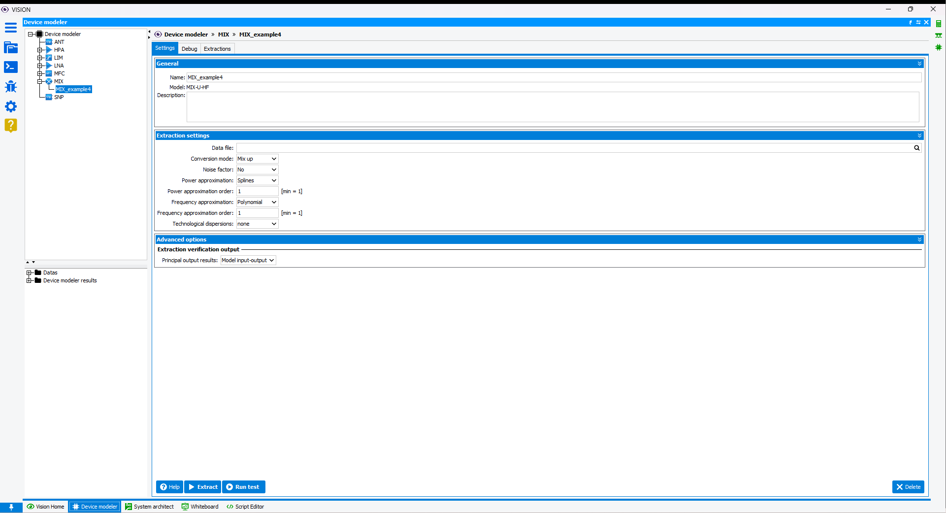
Workspace window.Figure: Extraction settings
Choose your data file
In the Extraction Settings
section, fill in the Data file field with the absolute or relative path
of your measurement or simulation file with the extension .dat. Click on Browser button to open the file browser and select your file in the local
file system. The file browser opens directly to the data directory specified
when creating the project.
Tune power and frequency approximation order parameters
Choose the conversion
mode according to the following configurations:
Mix down: IF = OL - RF;
Mix up: RF = OL - IF;
You have the option to add a noise factor file. In Power approximation order
and Frequency approximation order fields, start to put low orders and
checks results graphically after extraction.
Nota Bene:
The power approximation order can not be
greater than the number of power points included in the data file.
The frequency approximation can be carried out either by polynomial
function or by poles-residues decomposition. The polynomial approximation is
more adapted to weakly varying characteristics according to the frequency.
Otherwise, it is recommended to use poles-residues approximation.
The
frequency approximation order can not be greater than the number
of frequency points included in the data file. If exceeded, VISION will send
a message in the Output Console window and automatically truncate the
order of approximation to the maximum number allowed.
The
Technological dispersions option allows to specify a distribution
law of the gain (module) and phase shift characteristics of the amplifier.
Two laws of dispersion are possible (Uniform or Gaussian law). The
dispersion is characterized by two parameters: the standard deviation
Module, given in % of the nominal value for the gain, and the
standard deviation Phase in degrees for the phase shift.
Extract behavioral model and check with output graphs
Click on Extract button to start the extraction
process of the model. The output console is displayed:
The message Model Fit Error is showing the normalized mean square error
(NMSE) between data and model. Close the window to see in the
Applications window the number of the newly created extraction, here,
001. The results are saved and can visualized at any time by designating in the
tree the associated extraction. Click on the Output graphs tab to see
comparisons between data and model. Figure: Output graphs after MIX-U-HF model extraction 001
Various graphs are available to check the quality of the model according
to two dimensions: power and frequency. To examine the quality of the
approximation on the gain, select Volterra Model MIX-U-HF [Conversion
Gain] in Figures section and choose graphs you want to display in
Graphs section:
Tick dB[conv Gain] [par=Pin, LO freq] to display, for different
input powers and LO frequencies, the modulus of conversion gain in dB as
a function of dFreq, the offset between the central frequency of
the device characterization band and the frequency of the CW signal.
Tick phase[conv Gain] [par=Pin, LO freq] to display, for
different input powers and LO frequencies, the phase of conversion gain
in dB as a function of dFreq, the offset between the center
frequency of the device characterization band and the frequency of the
CW signal.
Tick dB[conv Gain] [par=Pin, Input freq] to display, for
different input powers and input frequencies, the modulus of conversion
gain in dB as a function of dFreq, the offset between the LO
central frequency of the device characterization band and the LO
frequency of the CW signal.
Tick phase[conv Gain] [par=Pin, Input freq] to display, for
different input powers and input frequencies, the phase of conversion
gain in dB as a function of dFreq, the offset between the LO
center frequency of the device characterization band and the LO
frequency of the CW signal.
Tick dB[conv Gain] [par=LO freq, Input freq] to display, for
different LO and input frequencies, the modulus of conversion gain in dB
as a function of Pin, the power of the CW input signal.
Tick phase[CW Gain] [par=LO freq, Input freq] to display, for
different frequencies, the phase of conversion gain in dB as a function
of Pin, the power of the CW input signal.
The graphs show the curves of data (from measurement or simulation) in red
lines and the extracted model in blue lines. The legend recalls the error NMSE
between model and data. If the number of curves makes the graphs unreadable,
click on Configure button to reduce the density of curves and/or limit the input
power range and frequency band.
Tune power and frequency range
If the first extraction is not satisfactory, it is necessary to increase the
order of approximation power and/or frequency.
Start by increasing the order of approximation power as long as the
error NMSE decreases significantly. Check graphically the comparison
between the data and the model.
Then, increase the order of approximation frequency as long as the error
NMSE decreases significantly. Check graphically the comparison between
the data and the model.
If the error is not small enough, restart in step a from the current
settings


 Browser button to open the file browser and select your file in the local
file system. The file browser opens directly to the data directory specified
when creating the project.
Browser button to open the file browser and select your file in the local
file system. The file browser opens directly to the data directory specified
when creating the project. 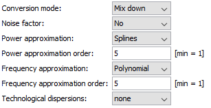

 Extract button to start the extraction
process of the model. The output console is displayed:
Extract button to start the extraction
process of the model. The output console is displayed: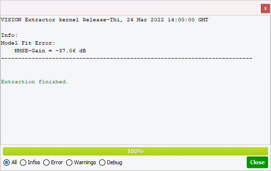 The message Model Fit Error is showing the normalized mean square error (NMSE) between data and model. Close the window to see in the Applications window the number of the newly created extraction, here, 001. The results are saved and can visualized at any time by designating in the tree the associated extraction. Click on the Output graphs tab to see comparisons between data and model.
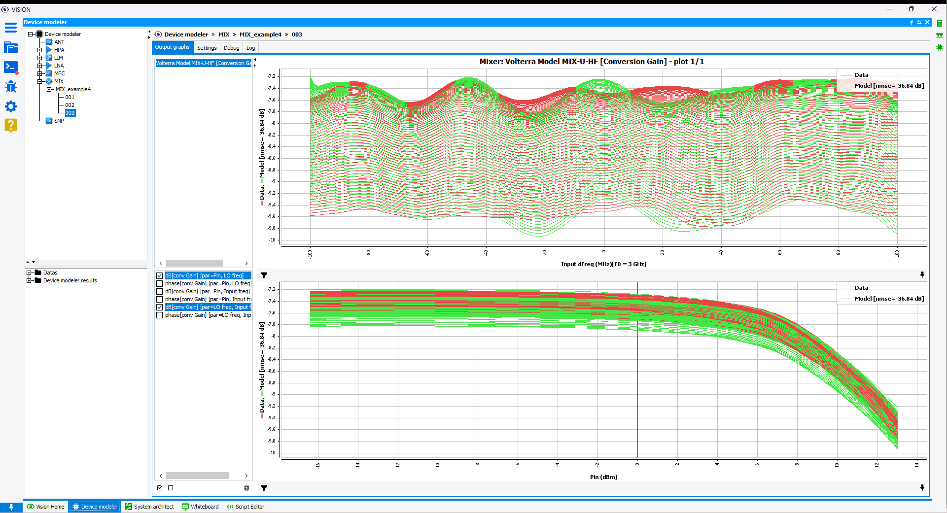
 Configure button to reduce the density of curves and/or limit the input
power range and frequency band.
Configure button to reduce the density of curves and/or limit the input
power range and frequency band.