How to extract Unilateral High Frequency memory (U-HF) model for limiter (LIM). The
LIM model is the simplest nonlinear amplifier model. Extracting this model requires little
information about the component, i.e. 1-tone CW measurements, performed on a nominal load
impedance. It therefore takes into account only the dispersive effects present in the
amplifier band and ignores other memory effects such as those due to polarization or
heating. Hence, it is suitable for applications processing signals with quasi-constant
envelope (frequency modulation), radar (frequency translation or slow amplitude variation,
low duty cycle). This model does not take into account load impedance changes.
An input file build from U-HF measurement data or U-HF simulation data. See
CW mode U-HF characteristics or "Simulation template
for U-HF data".
The basic steps for extract an U-HF model are:
Create a new LIM device
In an opened project, you can create a device from Applications window
or Workspace window.
From Applications window, right-click on Device modeler
and click on Create device. You can also right-click on
LIM and click on Create LIM device.
From Workspace window, click on Device modeler button,
select LIM and click on Open button then New
button.
The Create a new device dialog box is displayed. Figure: Create a new LIM device
In Type field, select LIM.
In Model field, select LIMITER.
In Name field, edit the name of your device. Here, we will name
it "LIM_example13".
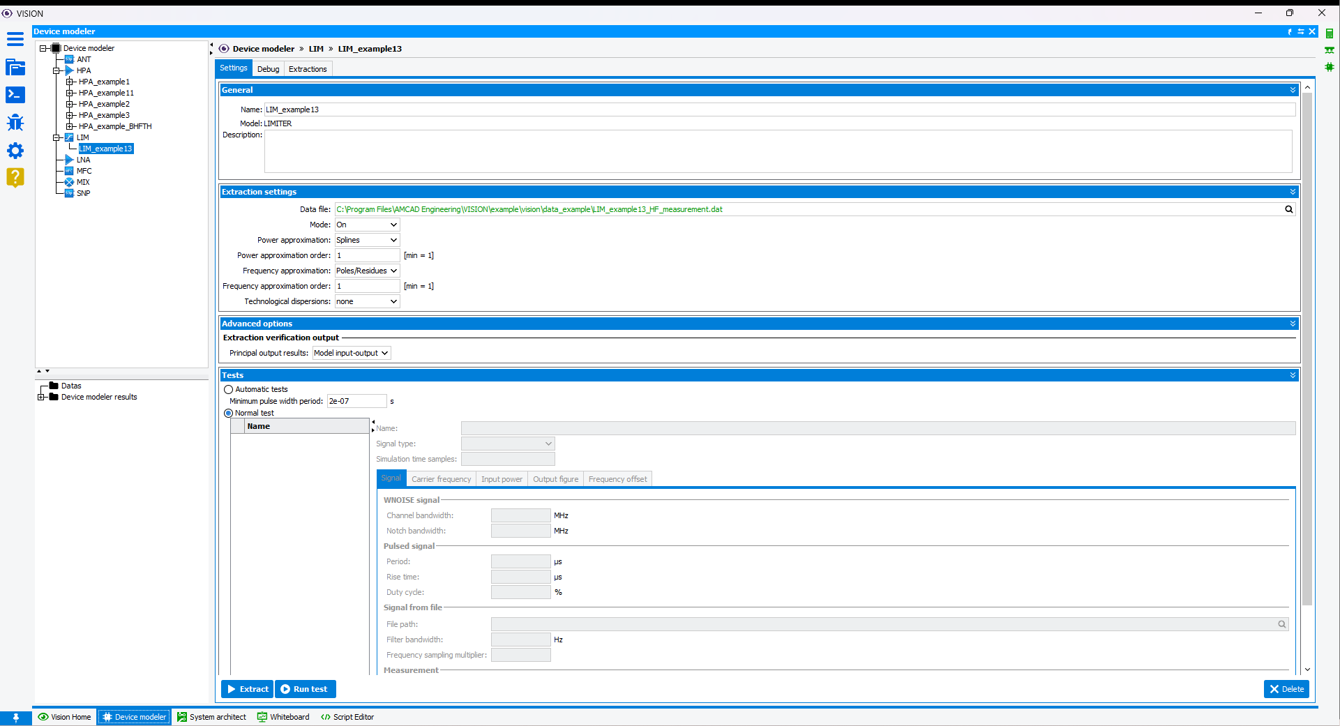
Click on Create button to display the new device in the tree of
Applications window and the settings of the extraction in
Workspace window.Figure: Extraction settings
Choose your data file
In the Extraction Settings section, fill in
the Data file field with the absolute or relative path of your
measurement or simulation file. Click on Browser button to open the file browser and select your file in the local
file system. The file browser opens directly to the data directory specified
when creating the project.
Tune power and frequency approximation order parameters
There are two ways to tune the
approximation order parameters:
If Power tuner order and Frequency tuner order options are
selected, VISION will automatically calculate power and frequency
approximation parameters.
In Power approximation order and Frequency approximation
order fields, start to put low orders and checks results
graphically after extraction.
Nota Bene:
In off mode, the limiter is a passive quadrupole that is best described
with an SNP model.
The
power approximation order can not be greater than the number of
power points included in the data file.
The frequency approximation
can be carried out either by polynomial function or by poles-residues
decomposition. The polynomial approximation is more adapted to weakly
varying characteristics according to the frequency. Otherwise, it is
recommended to use poles-residues approximation.
The frequency
approximation order can not be greater than the number of frequency
points included in the data file. If exceeded, VISION will send a message in
the Output Console window and automatically truncate the order of
approximation to the maximum number allowed.
It is recommended to
consider a frequency approximation in poles-residues if you are interested
in the transient response of the amplifier. In this particular case, you
must also take care to consider the order of poles-residues approximation as
low as possible (do not seek a perfect fit of the frequency characteristics
by pushing the order of approximation to the maximum).
The
Technological dispersions option allows to specify a distribution
law of the gain (module) and phase shift characteristics of the amplifier.
Two laws of dispersion are possible (Uniform or Gaussian law). The
dispersion is characterized by two parameters: the standard deviation
Module, given in % of the nominal value for the gain, and the
standard deviation Phase in degrees for the phase shift.
Extract behavioral model and check with output graphs
Click on Extract button to start the extraction
process of the model. The output console is displayed:
The message Model Fit Error is showing the normalized mean square error
(NMSE) between data and model. Close the window to see in the
Applications window the number of the newly created extraction, here,
001. The results are saved and can visualized at any time by designating in the
tree the associated extraction. Click on the Output graphs tab to see
comparisons between data and model. Figure: Output graphs after LIM model extraction 001
Various graphs are available to check the quality of the model according
to two dimensions: power and frequency. To examine the quality of the
approximation on the gain, select Volterra Model HPA-U-HF [1Tone CW Gain]
in Figures section and choose graphs you want to display in Graphs
section:
Tick dB[CW Gain] [par=Pin] to display, for different input power,
the modulus of gain in dB as a function of dFreq, the offset
between the central frequency of the device characterization band and
the frequency of the CW signal.
Tick phase[CW Gain] [par=Pin] to display, for different input
power, the phase of gain in dB as a function of dFreq, the offset
between the center frequency of the device characterization band and the
frequency of the CW signal.
Tick dB[CW Gain] [par=Freq] to display, for different
frequencies, the modulus of gain in dB as a function of Pin, the
power of the CW input signal.
Tick phase[CW Gain] [par=Freq] to display, for different
frequencies, the phase of gain in dB as a function of Pin, the
power of the CW input signal.
The graphs show the curves of data (from measurement or simulation) in red
lines and the extracted model in blue lines. The legend recalls the error NMSE
between model and data. If the number of curves makes the graphs unreadable,
click on Configure button to reduce the density of curves and/or limit the input
power range and frequency band.
Tune power and frequency range
If the first extraction is not satisfactory, it is necessary to increase the
order of approximation power and/or frequency.
Start by increasing the order of approximation power as long as the
error NMSE decreases significantly. Check graphically the comparison
between the data and the model.
Then, increase the order of approximation frequency as long as the error
NMSE decreases significantly. Check graphically the comparison between
the data and the model.
If the error is not small enough, restart in step a from the current
settings
The user can find in the following table an example of the extraction process.
Here, the parameters of extraction 008 allow to have the smallest error between
the data and the model.
Table 1. Extraction settings HPA_example1
Extraction
Power approximation order
Frequency approximation order
NMSE (dB)
001
1
1
-23.09
002
2
1
-23.37
003
1
2
-23.09
004
1
3
-23.09
005
1
4
-23.09
006
2
4
-23.38
007
2
5
-23.36
008
3
5
-23.36
009
4
5
-23.27
Figure: Output graphs after LIM model extraction 008
You can label an extraction as a reference to differentiate it from others
for use in System Architect. To do so, select the appropriate extraction of your
device in the Applications , right-click on it, and subsequently select
the add to favourites option.
Apply a test plan
It is recommended to perform basic simulations after an extraction to check
the behavior of the model in the face of signals different from those used for
its identification. VISION provides tools to simply configure signals and
perform simulations directly after model extraction. In Applications
window, click on your device, here HPA_example1, to show up
Settings tab in the Workspace window. Click on Test
plan section to reveal two options:
Automatic tests: this option allows you to perform simulations
with 2-tone and pulse signals whose settings are set automatically,
except for the pulse width period.
Normal test: this option allows simulations with CW, 2-tone,
pulse and white noise signals. You can also provide your own IQ file by
specifying the path of the file.Figure: Test plan window
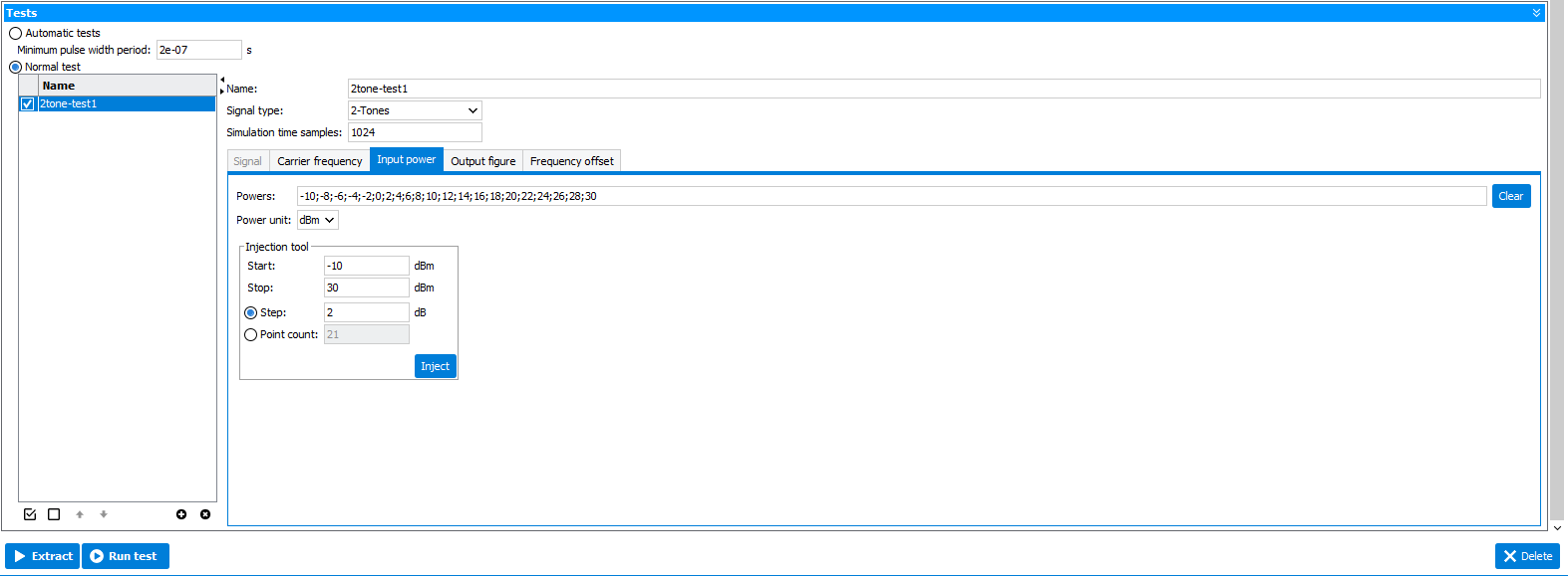
To set up a test, select Normal test and click on New test button. A new test is added to the
list with the default name "test1". Then, the test highlighted in blue can be
configured. Here, a configuration example of 2-tone test:
Name: 2tone-test1
Signal type: 2TONE
Number of samples: 1024
Carrier frequency: 9.75 GHz
Power sweep: -10 to 30 dBm with 2 dBm step
Output figure: IMD3
Frequency sweep: 1 to 161 MHz with 1 MHz step
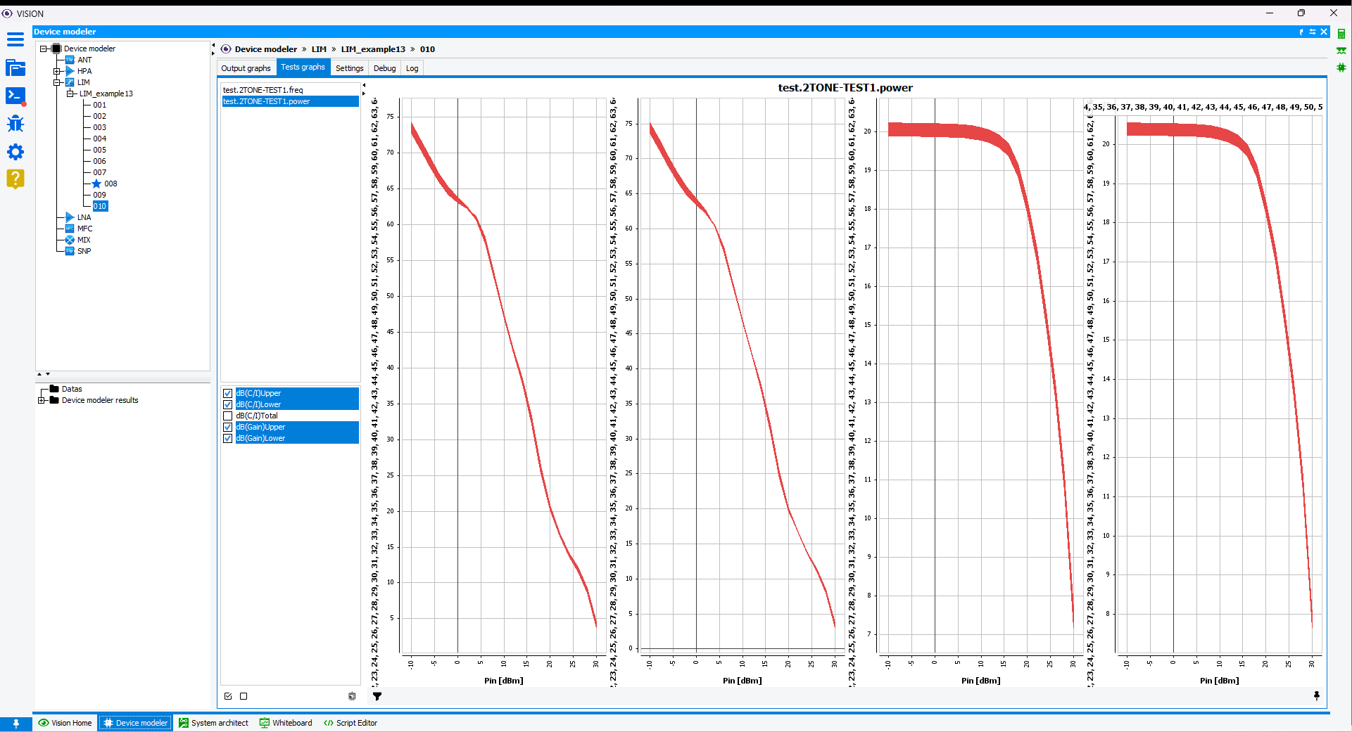
Tick your newly configured test in the list and click on Extract button to run the test after the extraction process. The
simulation results are saved and can visualized at any time by designating in
the tree the associated extraction. Click on the Test graphs tab to see
IMD3 results according to frequency and power.


 Browser button to open the file browser and select your file in the local
file system. The file browser opens directly to the data directory specified
when creating the project.
Browser button to open the file browser and select your file in the local
file system. The file browser opens directly to the data directory specified
when creating the project. 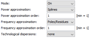
 Extract button to start the extraction
process of the model. The output console is displayed:
Extract button to start the extraction
process of the model. The output console is displayed: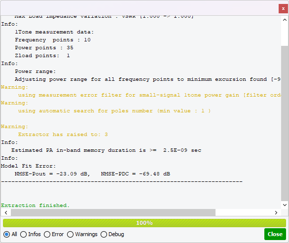 The message Model Fit Error is showing the normalized mean square error (NMSE) between data and model. Close the window to see in the Applications window the number of the newly created extraction, here, 001. The results are saved and can visualized at any time by designating in the tree the associated extraction. Click on the Output graphs tab to see comparisons between data and model.
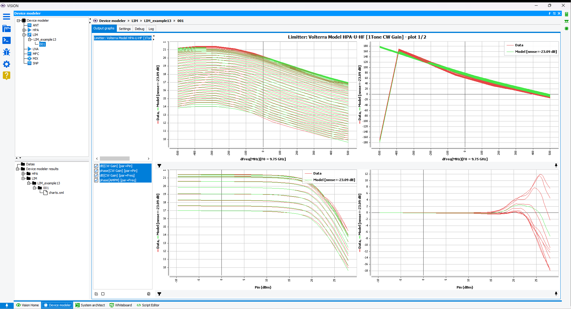
 Configure button to reduce the density of curves and/or limit the input
power range and frequency band.
Configure button to reduce the density of curves and/or limit the input
power range and frequency band. 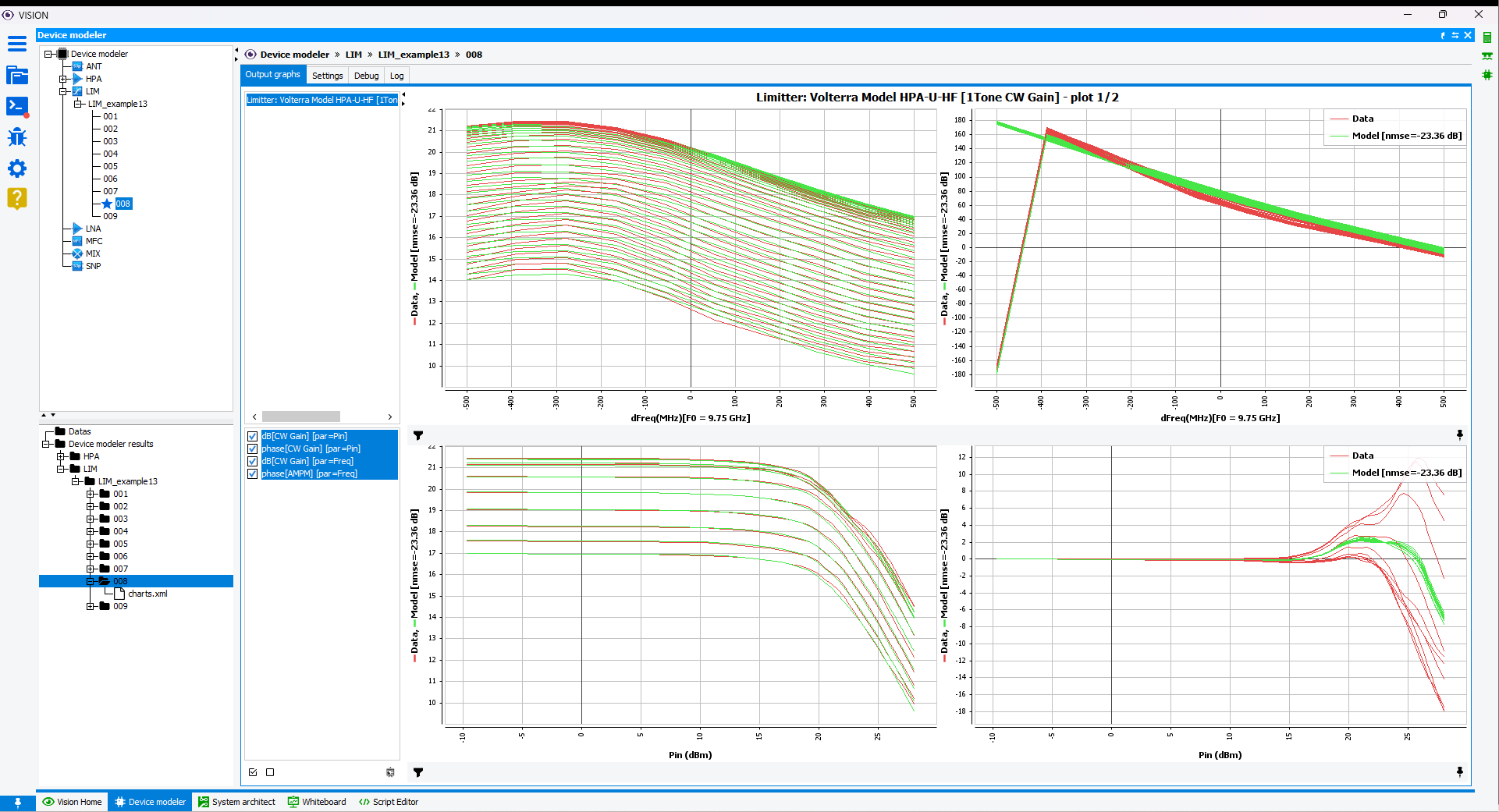
 New test button. A new test is added to the
list with the default name "test1". Then, the test highlighted in blue can be
configured. Here, a configuration example of 2-tone test:
New test button. A new test is added to the
list with the default name "test1". Then, the test highlighted in blue can be
configured. Here, a configuration example of 2-tone test: