Co-simulation with system modeler
This section describe how to perform a co-simulation between COMLIB2 and the Vision System modeler. A CW simulation in COMLIB is perform in order to illustrate this process. Vision model are advanced model witch take into account dispersive and non linear phenomena. For dispersive component this lead to transient response estimation at time equal to 0 seconds. User may take into account an amount of time which correspond to transient time before analysed real continuous response of the system.
To begin this task, you will need:
- A licence of VISION Comlib Simulator. See Installation and licence setup.
- A licence of VISION System modeler Simulator.
The basic steps to perform a CW simulation are:
-
Drag and drop the Template for Co-simulation block from the
palette window in Template schematics section to the
schematic window.
Figure: CW Co-simulation template 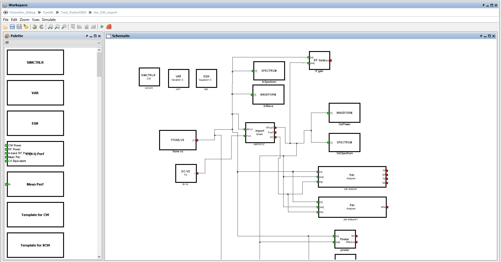
This template is very similar from Perform CW simulation, the difference is the use of block Import model. Double-click on the Import model block to open the Parameters window. Fill the data file directory in order to match with directory of the model export made in system modeler Perform model export. -
The block import model has polymorphism property. This stands that it has the
property to change its appearance according to the model input/output which has
been exported in system modeler. At this step user can verify the information
automatically fill by the block are true and match with these use in Perform model export.
Figure: Import Model Interface 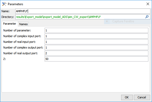
One can note this is a RF device model which has 1 complex input port (RF input envelope), 1 complex output port (RF output envelope), 1 real input port (Input carrier frequency), 1 real output port (Output carrier frequency) and one additional parameter set by default to 50.0 (Zload). -
The following step is to compare the behavior of the model in System modeler
and in Comlib2. We will set the parameters of the source 1Tone-VS. Double
click on the1Tone-VS block to open the Parameters window and set
the amplitude, frequency and phases of the CW signal provided by the source.
Here, we set a parameter P as value of amplitude (Phase is equal to zero).
Figure: 1 Tone Vs Parameters 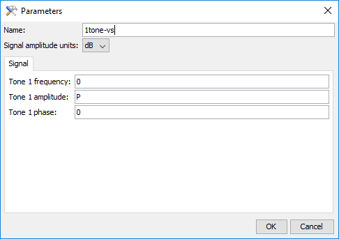
-
According to the Perform model export
we choose to sweep the power from -30 dBm to 15 dBm. The carrier frequency is
fixed to 0.83e9 and the load is swept from 20 to 100 Ohms.
Figure: Variable definition 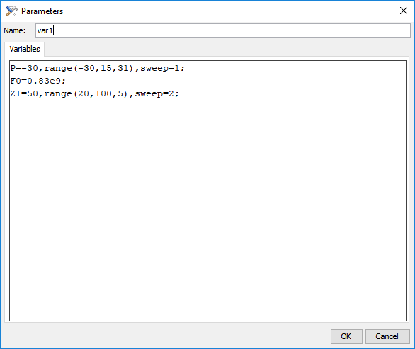
-
In this step we will define time parameters of the Data Flow simulation
Controller. The choice made here is a total bandwidth of 100 MHz with a
resolution of 1 MHz which define 100 temporal points (100e6/1e6) and a
simulation time of 100/500e6 = 2e-7 sec
Figure: Equation Definition 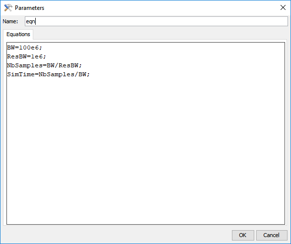
-
We can now edit following probes Pmeter, Pdc analyser, Waveform, Spectrum, One can, note that for a
convenient scaling of Pdc analyser results it is adapted to have 2 blocks : one
for efficiency ,second one for Pdc. In the following graph we can see Pdc
analyser and Pmeter results.
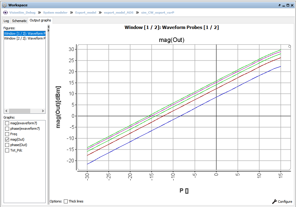
Figure: Output Results from Comlib2 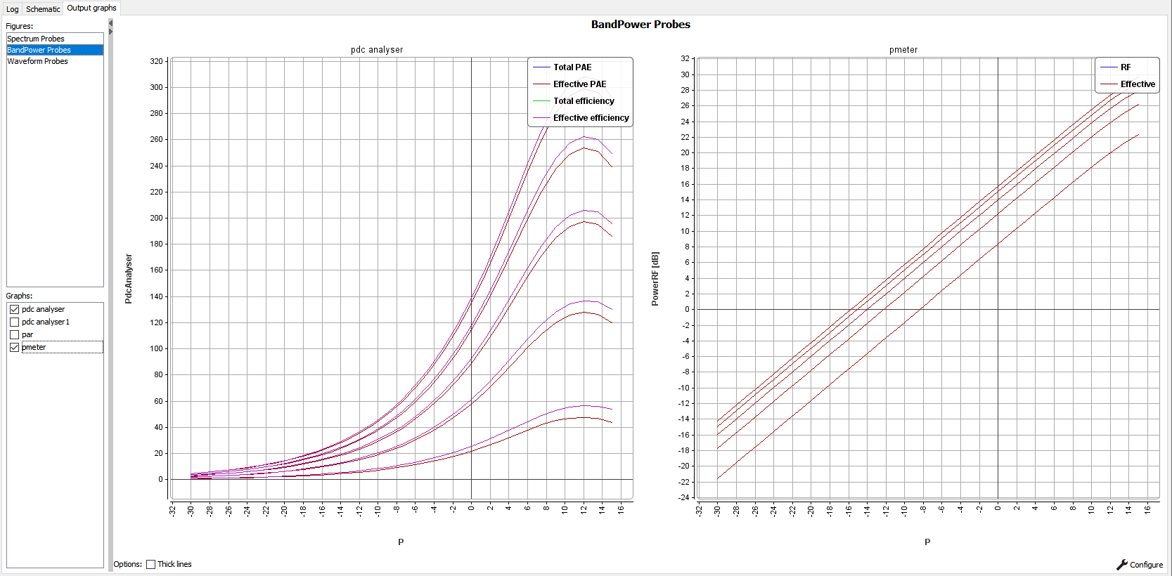
If we compare the power plotted in System modeler we can observe the following display which show same results in the 2 simulation platform.Figure: Output power results from system modeler