Use an imx file generated from VISION simulation

How to display data generated from VISION simulation using System Architect

1. Open Whiteboard application available in the Plug-in manager button in the left side of VISION application.

   
   

   

   
   

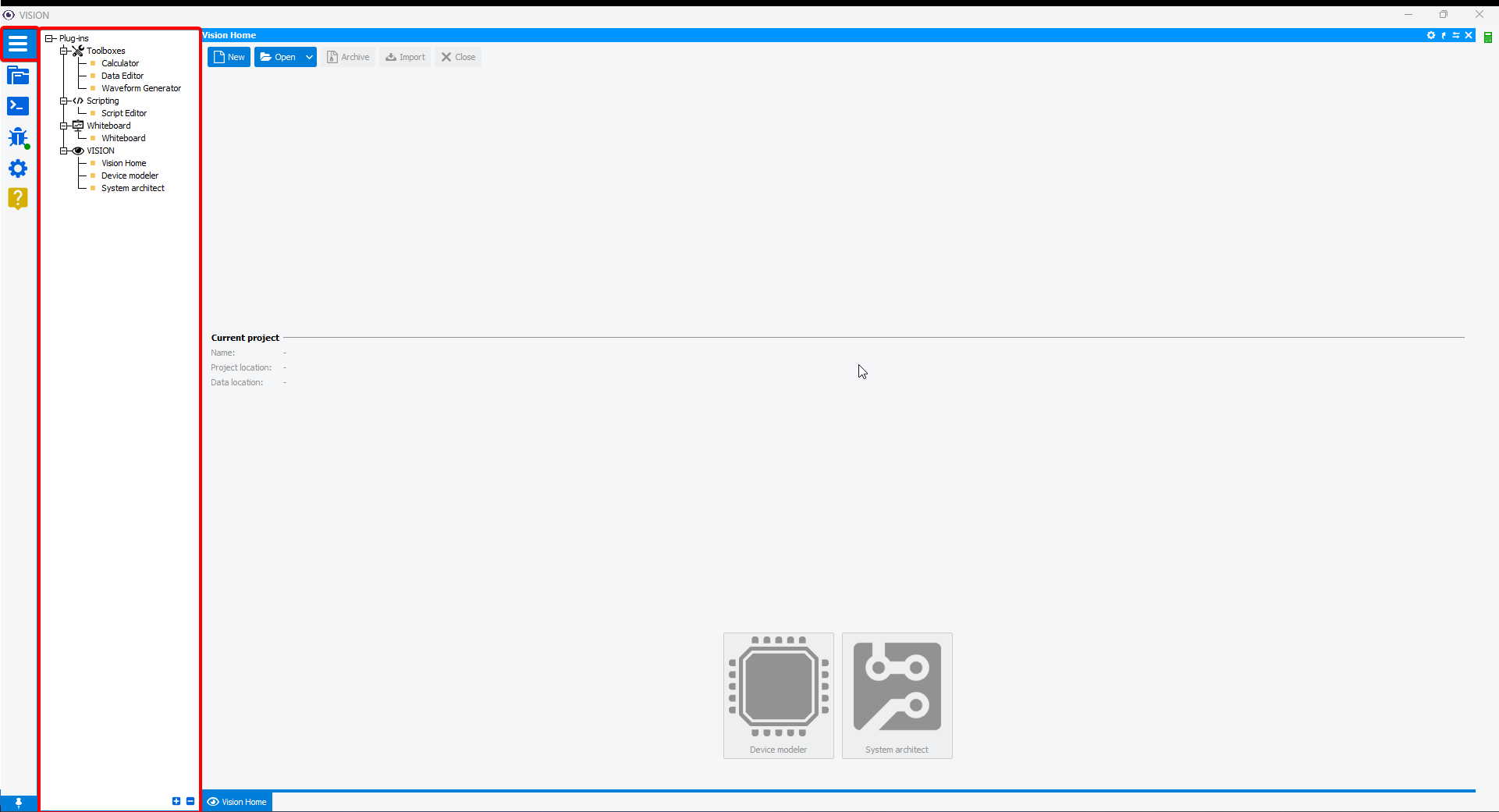
2. Open a whiteboard project and display the Whiteboard Tools panel.

   
   

   

   
   

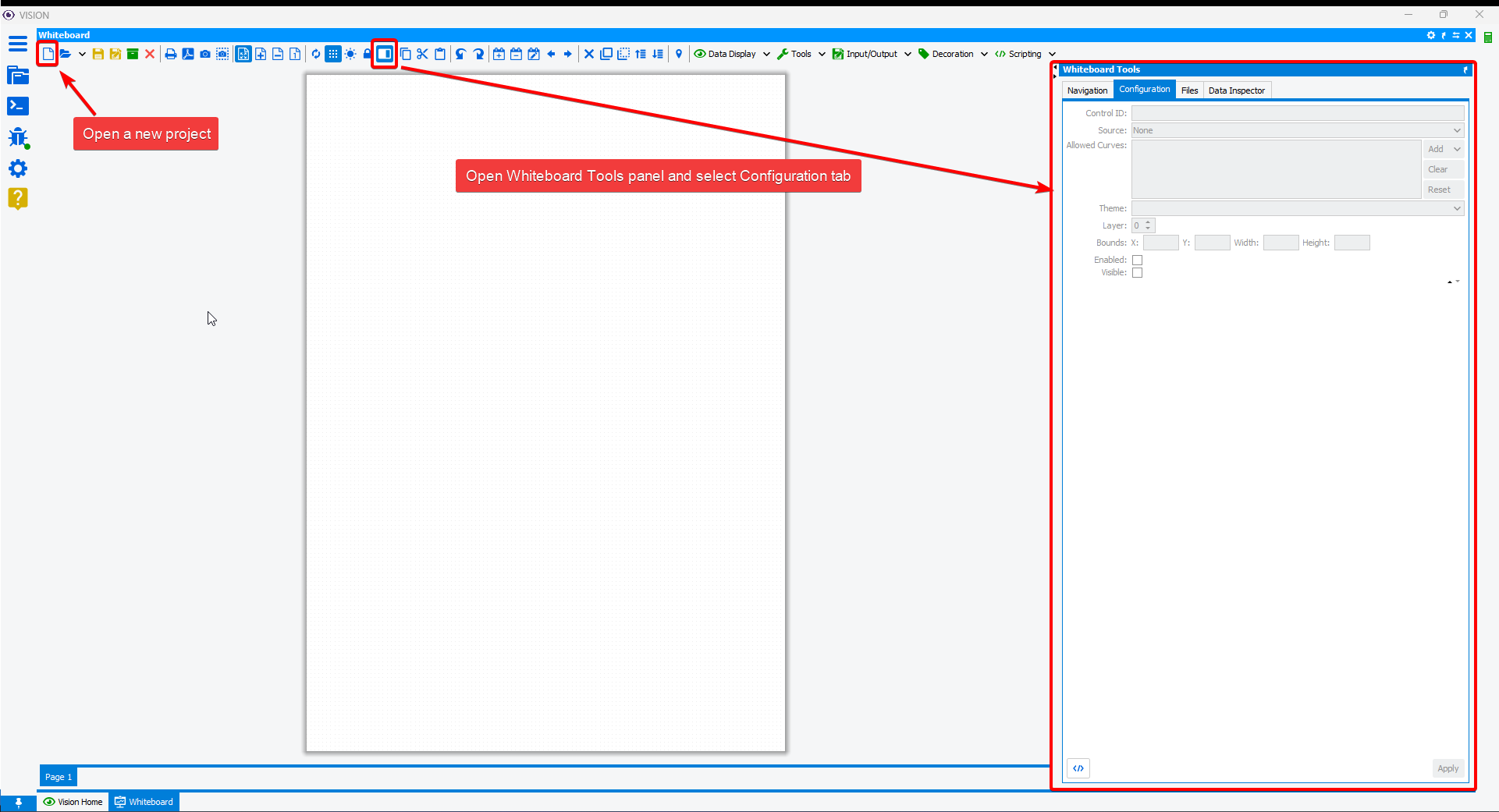
3. Click on Data manager and open the imx file "sim_test.imx".

   
   

   

   
   

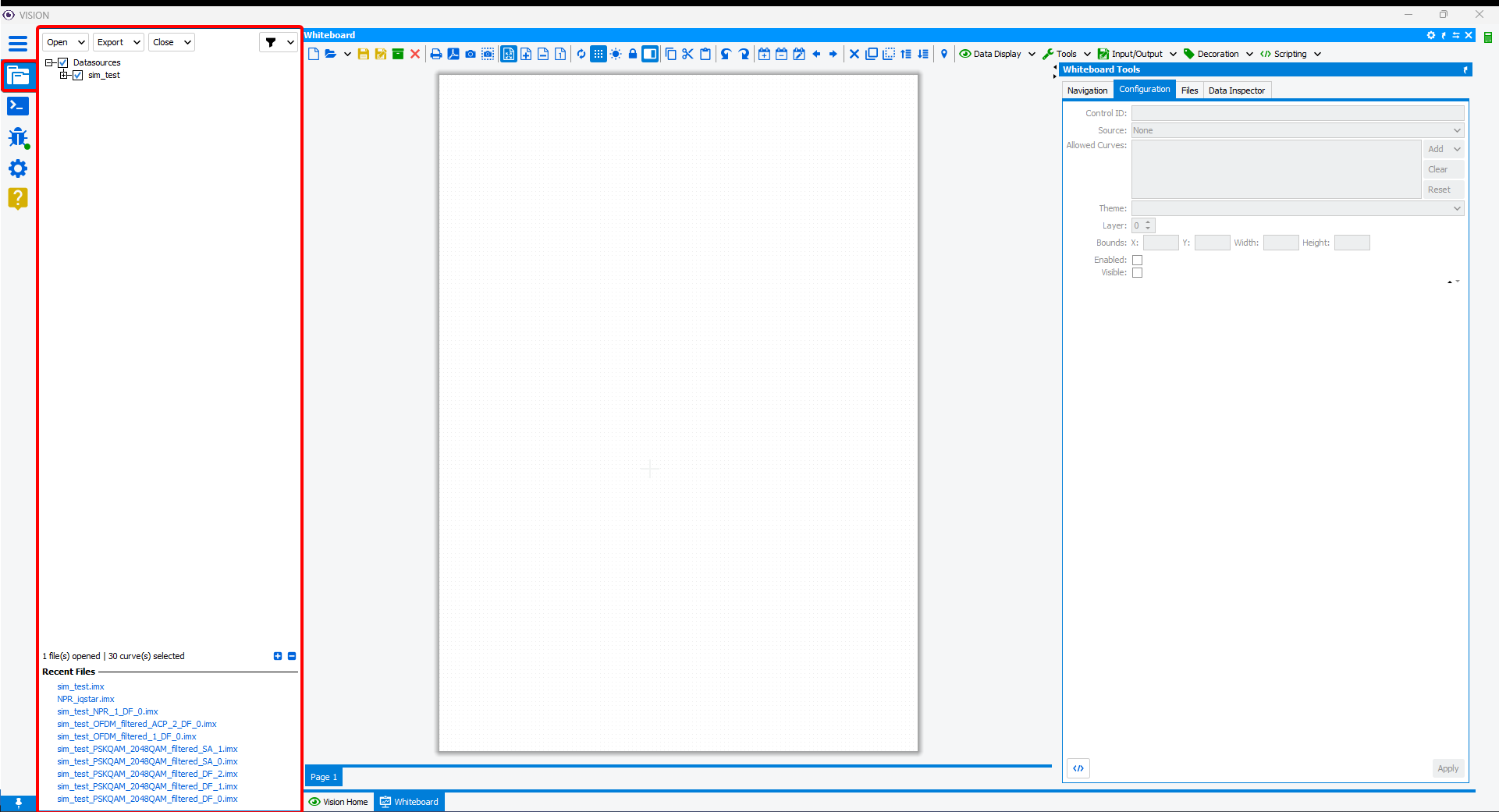
4. In the menu bar, click on Data Display then Graph and draw a box in Page 1 to display a graph. In the Data manager panel select only probe_iq dataset.

   
   

   

   
   

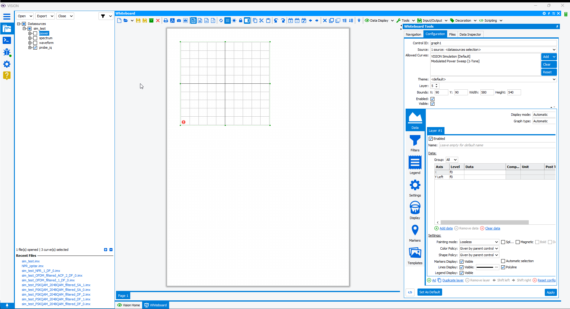
5. In the Whiteboard Tools panel, Configuration tab is available to setup graph1 parameters corresponding to the displayed graph. Basic configuration is as follows:
   • Control ID: this field is used to assign an ID name to the graph to locate it in the project or control it from a script.
   • Source: This feature allows you to select the data sources that will be processed by the graph. By default, "<datasources selection>" is chosen and corresponds to what is in the Data manager panel.
   • Allowed Curves: Depending on the data selected in the source option, the tool automatically recognises the file formats compatible with the whiteboard and lists them here. Press the Reset button to refresh and check the types of format available from the sources. Here, "Modulated Power Sweep [1-Tone]" is displayed, corresponding to the format of the "probe_iq" dataset selected in the Data manager.
   • Data section: This section allows you to select the data to be displayed and set the curve display parameters. Click on the table to display figures of merit related to IQ signal analysis computed thanks to IQ_PROBE block in System Architect (see Perform Transient simulation using IWF file and IQ probe). Here, select data to display "ACPR 1 Lower" vs "Pin Available" in dBm.

   
   

   

   
   

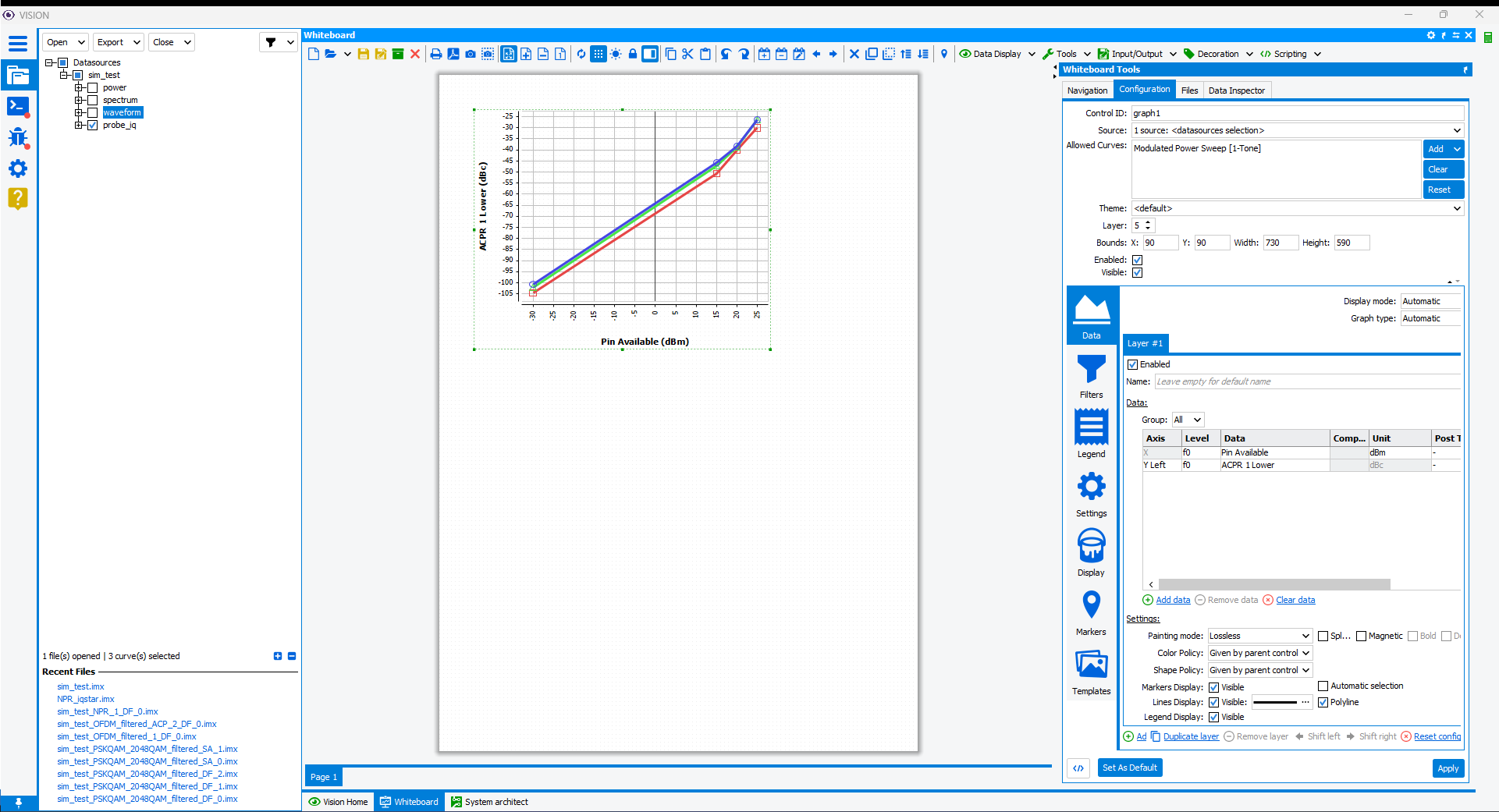
6. Click on any data point in Graph 1 and create another graph in Page 1. Configuration tab is updated to setup the new graph named graph2. Select in the Source option graph1 and deselect <datasources selection>. Allowed Curves section is updated by displaying the format corresponding to the subcurves data generated from Graph 1.

   
   

   

   
   

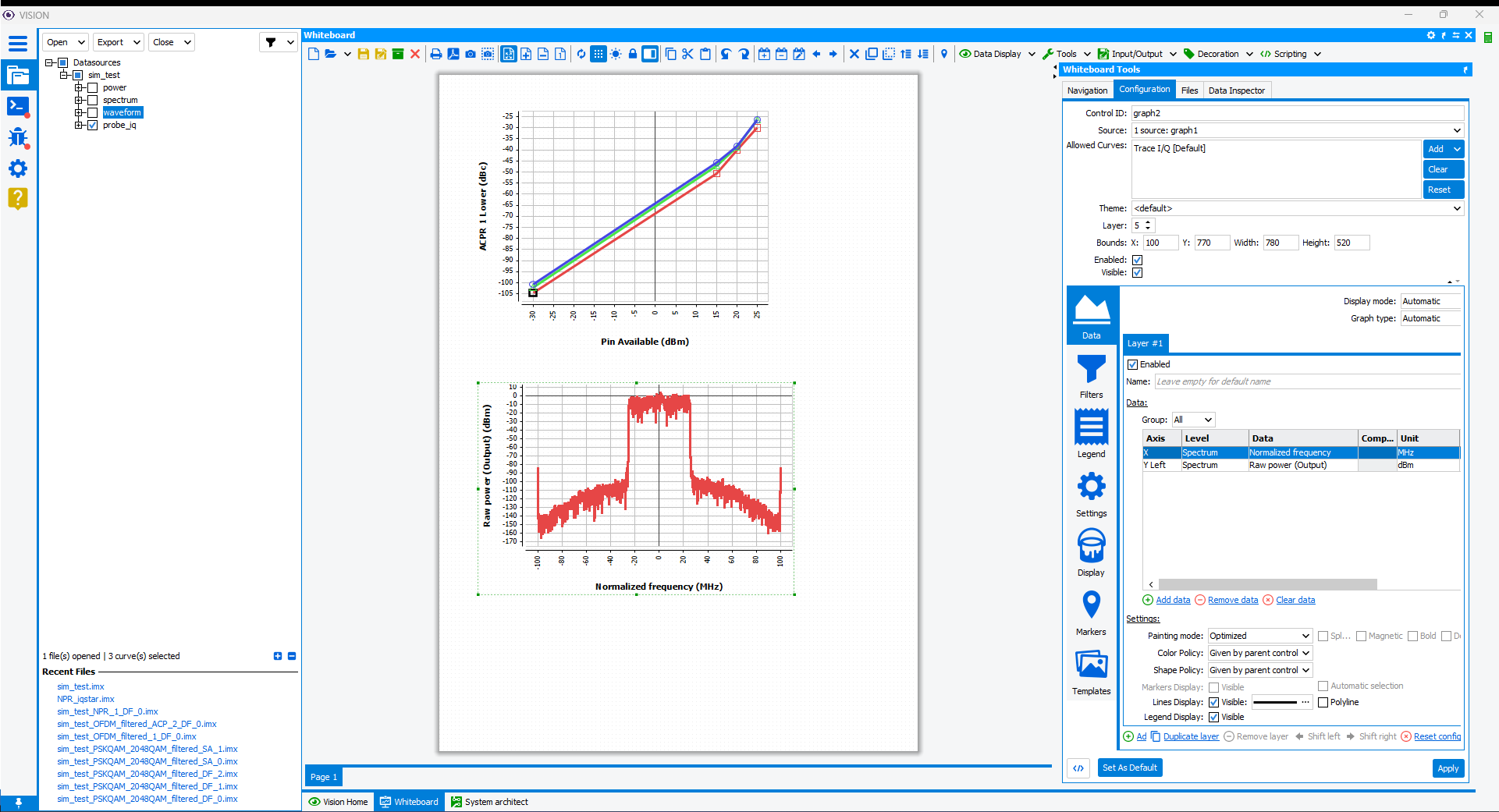
7. In Configuration tab from Whiteboard Tools panel, select data to display related to the item selected in Graph 1. Subcurve data are categorized thanks to Level column: I/Q, CCDF, Spectrum etc... Select Spectrum as Level and display Output spectrum by selecting Normalized frequency vs. Raw power (Output). In Painting mode option, select Optimized to get a nice display of the spectrum.